
3.10. Case Studies
We present three case studies, all involving FEA for structural analysis. The first case, sizing optimization of roadwheel, aims to minimize volume and constrain deformation of a tracked-vehicle roadwheel by varying its thicknesses. The second case study optimizes the geometric shape of an engine connecting rod using a p-version FEA code. The third case study focuses on optimizing the geometric shape of an engine turbine blade parameterized in Pro/ENGINEER.
3.10.1. Sizing Optimization of Roadwheel
In this case study, we present a sizing optimization for a tracked-vehicle roadwheel, in which thicknesses of shell finite elements are varying for better designs. Function evaluations are carried out using FEA, in which shell elements (instead of solid elements) are created from the surface geometric model created in a geometric modeling tool, MSC/PATRAN (www.mscsoftware.com/product/patran).
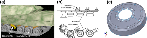
The roadwheels shown in Figures 3.26a and b are heavy load carrying components of the tracked vehicle suspension system. There are seven wheels on each side of the vehicle. The geometric model of the roadwheel is created in MSC/PATRAN as quadrilateral surface patches, as shown in Figure 3.26c. The objective of this design problem is to minimize its volume with prescribed allowable deformation at the contact area, by varying its thicknesses.
3.10.1.1. Geometric modeling and design parameterization
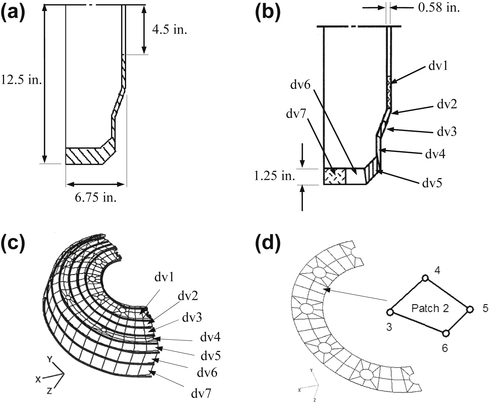
Due to symmetry, only half of the wheel is modeled for design and analysis. The outer diameter of the wheel is 25 in., with two cross-section thicknesses, 1.25 in. at rim section (dv5, dv6, and dv7) and 0.58 in. at hub section (dv1 to dv4), as shown in Figure 3.27a. To model the wheel, 216 Coons patches and 432 triangular finite elements are created in the geometric and finite element models, respectively, using PATRAN.
Thicknesses of the wheel are defined as design variables, which are linked with surface patches along the circumferential direction of the wheel to maintain a symmetric design, as illustrated in Figures 3.27b and c. Figure 3.27d shows patches along the inner edge of the wheel, in which patch thicknesses are linked together as design variable dv1. In a similar fashion, addition six design variables are defined for the wheel, as shown in Figures 3.28b and c. In the current design, we have dv1 = dv2 = dv3 = dv4 = 0.58 in., and dv5 = dv6 = dv7 = 1.25 in.
3.10.1.2. Analysis model
ANSYS plate elements STIF63 are employed for finite element analysis. There are 432 triangular plate elements and 1650 degrees of freedom defined in the model, as shown in Figure 3.28a. This wheel is made up of aluminum with modulus of elasticity, E = 10.5 × 10⁶ psi, shear modulus, G = 3.947 × 10⁶ psi, and Poisson's ratio, v = 0.33.
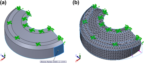
The circumference of the six small holes in the hub area is fixed. Symmetric conditions are imposed at the cutoff section, and a distributed load of total 12,800 lb is applied to the six elements in the area where the wheel contacts the track. A deformed wheel shape, obtained from ANSYS analysis results, is displayed in PATRAN for result evaluation, as shown in Figure 3.26b. From the analysis results, it is found that the maximum displacement occurs at contact area, more specifically node 266, in the y-direction with magnitude 0.108 in. Volume of the wheel is 361.9 in3.
3.10.1.3. Performance measures
The maximum displacement (found at 266 in the y-direction) and wheel volume are defined as performance measures for the design problem.
3.10.1.4. Design sensitivity results and display
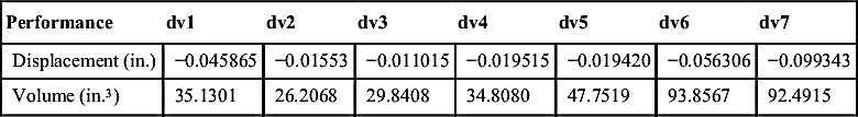
In this case, gradients of the displacement and volume are calculated using the sensitivity analysis method based on the continuum formulation to be discussed in Chapter 4. Design sensitivity coefficients computed are listed in Table 3.2.
To display design sensitivity coefficients, both a PATRAN fringe plot and bar chart are utilized. Figure 3.29 shows the design sensitivity coefficients of the displacement performance measure. The design sensitivity plots clearly indicate that increasing the thickness at outer edge of the wheel; that is, design variable dv7 reduces the displacement most significantly. As shown in the bar chart, a 1-in. increment of thickness at outer edge of the wheel yields a 0.0993 in. reduction in the displacement. This influence decreases from the outer to inner edges of the wheel. At the inner edge of the wheel, the influence is increasing to about 40% of the maximum value.
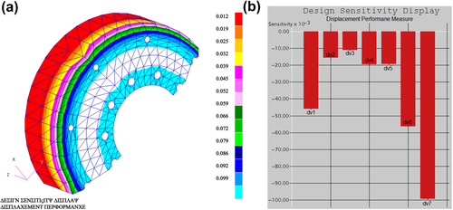
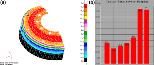
Figure 3.30 shows the design sensitivity coefficients of the volume performance measure. The result shows that increasing thickness around outer edge of the wheel, dv6 and dv7, increases the volume performance measure most significantly. As shown in the bar chart, a 1-in increment of thickness around the outer edge of the wheel yields 93.4 in.3 and 92.5 in.3 gain in wheel volume. The rate of influence decreases from the outer to inner edges of the wheel.
3.10.1.5. What-if study
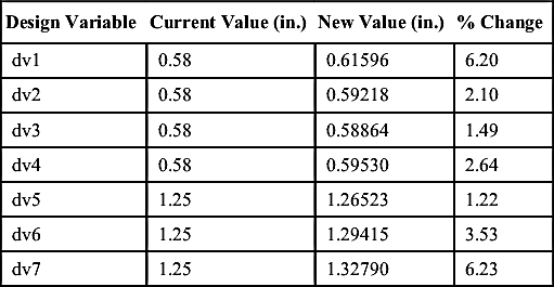
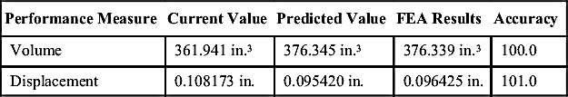
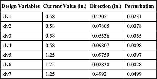
A what-if study is carried out based on the steepest descent direction of the displacement performance measure with a step size of 0.1 in. The design direction shown in Table 3.3 suggests the most effective design change to reduce the maximum deformation at node 266. Table 3.4 shows the first-order prediction of displacement and volume performance values using the design sensitivity coefficients and design perturbation. It is shown that the displacement performance is reduced from 0.1082 to 0.0954 in., following such a design change. However, volume increases from 361.94 to 376.35 in.3. A finite element analysis is carried out at the perturbed design to verify if the predictions are accurate. The finite element analysis results given in Table 3.4 show that the predicted performance values are very close to the results from finite element analysis because the sensitivity coefficients are accurate and the design perturbation is within a small range.
3.10.1.6. Trade-off determination
From the design sensitivity displays and what-if study, a conflict is found in the design in reducing structural volume and maximum deformation. To find the best design direction, a trade-off study is carried out. To support the trade-off study, the volume performance measure is selected as the objective function, and the displacement performance measure is defined as constraint function, with an upper bound of 0.1 in. Notice that, in the current design, the displacement performance measure is 0.1082 in., which is greater than the bound. Therefore, the current design is infeasible. The side constraints are defined for all the design variables with bounds 0.1 and 10.0 in.
With an infeasible design, the second option, constraint correction, is selected for trade-off study. A QP subproblem is formed and solved to determine a design direction. Table 3.5 shows the design direction obtained from solving the QP subproblem.
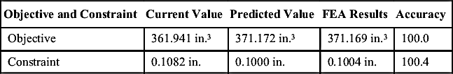
A what-if study is carried out again following the design direction suggested by the trade-off determination, using a step size 0.1 in. The results of the what-if study are listed in Table 3.6, which show the approximation of objective and constraint function values using the design sensitivity coefficients and design perturbation. In this case, constraint violation is completely corrected with a small increment in the objective function (volume). A finite element analysis is carried out at the perturbed design to verify the approximations are accurate, as given in Table 3.6.
3.10.1.7. Design optimization
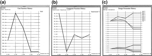
To perform design optimization, the same objective, constraint, and side constraints defined in trade-off determination are used. DOT, ANSYS, and sensitivity computation and model update programs similar to those discussed in Section 3.8.2 are integrated to perform design optimization. After four iterations, a local minimum is achieved. The optimization histories for objective, constraint, and design variables are shown in Figures 3.31a, b, and c, respectively.
From Figure 3.31a, the objective function starts around 362 in.3 and jumps to 382 in.3 immediately to correct constraint violation. Then, the objective function is reduced further until a minimum point, 354 in.3 is reached. Also, the constraint function history graph shows that 80% violation is found at the initial design, and the violation is reduced significantly to 65% below the bound at the first iteration. Then, the constraint function is stabilized and stays feasible for the rest of iterations. At optimum, the constraint is 4% below the bound, the maximum displacement becomes 0.09950 in., and the design is feasible. The most interesting observation is that, from Figure 3.31c, all design variables are decreasing in the design iterations, except for dv1 and dv7. Design variable dv1 increases from 0.58 to 0.65 in. at the optimum. However, the most significant design change is dv7 from 1.25 to 1.44 in., which contributes largely to the reduction in the deformation, as listed in Table 3.7. Decrement of the rest of the design variables contributes to the volume reduction.
3.10.1.8. Postoptimum study
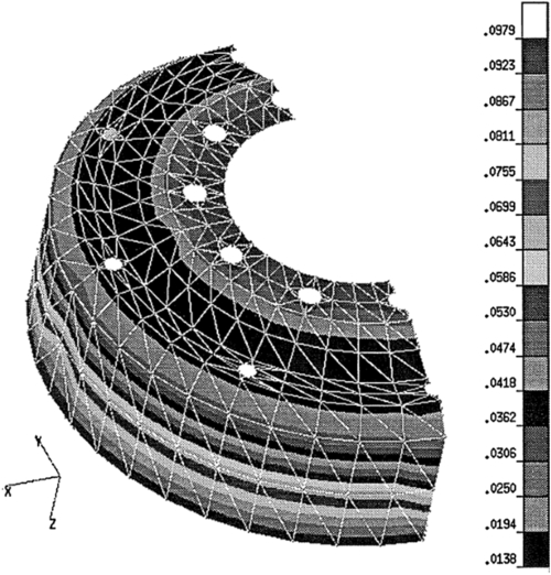
At optimum, the designer can still acquire significant information to assist in the design or manufacturing process. The design sensitivity plot for a displacement performance measure at optimum is shown in Figure 3.32. The sensitivity plot shows that thickness at the outer edge has a significant effect on the maximum displacement at the contact area. In other areas, sensitivity coefficients are relatively small. This plot suggests that in the manufacturing process, restrictive tolerance needs to be applied to the thickness at the outer edge because small errors made in the outer rim will impact the displacement.
3.10.2. Shape Optimization of the Engine Connecting Rod
This case study involves shape optimization of an engine connecting rod, in which the geometric shape of the rod is parameterized to achieve an optimal design considering essential structural performance measures, such as stresses. In this case, geometric and finite element models are created in a p-version FEA code, called STRESSCHECK (www.esrd.com). FEA is performed also using STRESSCHECK. Shape design sensitivity computation is carried out using the continuum-based method to be discussed in Chapter 4, and optimization is carried out using DOT. STRESSCHECK and DOT are integrated with the sensitivity analysis code to support a batch mode optimization for this example.
3.10.2.1. Geometric and finite element models
The connecting rod is modeled as plane stress problem using 25 quadrilateral p-elements. The shape of the connecting rod is to be determined to minimize its weight subject to a set of stress constraints. The geometric model, finite element mesh, physical dimensions, and design variables are shown in Figure 3.33. The material properties are modulus of elasticity E = 2.07 × 10⁵ MPa and Poisson's ratio v = 0.298.
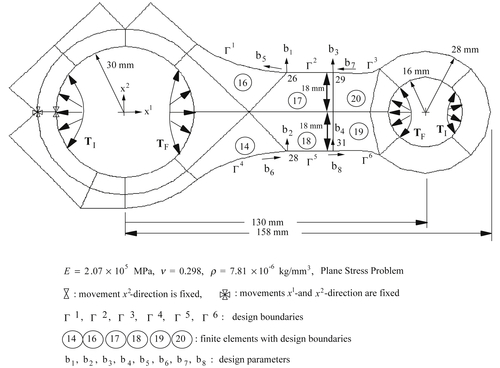
In this problem, two loadings are considered: the firing load TF, which occurs during the combustion cycle, and the inertia load TI, which occurs during the suction cycle of the exhaust stroke. These loads are defined as follows (Hwang et al. 1997):
 (3.98)
 (3.99)
where θ is the angle measured counterclockwise from the positive x1-axis.
3.10.2.2. Design parameterization and problem definition
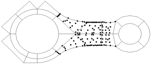
A design boundary that consists of boundary segments Γ1 to Γ6 is parameterized using Hermit cubic curves. Eight design variables are shown in Figure 3.33 and listed in Table 3.8. For the firing load, the upper bound of the allowable principal stress is σUF = 37 MPa, and the lower bound is σUF = −279 MPa. For the inertia load, the upper bound of the allowable principal stress is σUI = 136 MPa, and the lower bound is σUI = −80 MPa. There are 488 stress constraints imposed along boundaries Γ1 to Γ6 and at the interior of elements 14, 16, 17, 18, 19, and 20, as shown in Figure 3.34.
3.10.2.3. Design optimization
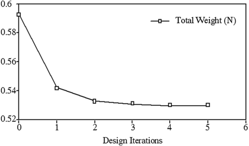
At the initial design, the total weight of the rod is 0.5932 N and no stress constraints are violated. For design optimization, the modified feasible direction method of DOT is used. After five design iterations, an optimum design is obtained. The total weight at the optimum design is 0.5298 N. The objective function history is shown in Figure 3.35. The total weight has been reduced by 10.7%. Because the firing load is larger than the inertia load, a number of stress constraints are active under the firing load at the optimum design. Figures 3.36 and 3.37 are the stress contours at the initial and optimum designs, respectively. As shown in Figure 3.37, all active stress constraints are due to the firing load.
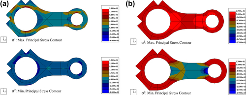
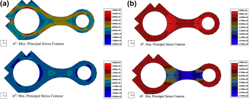
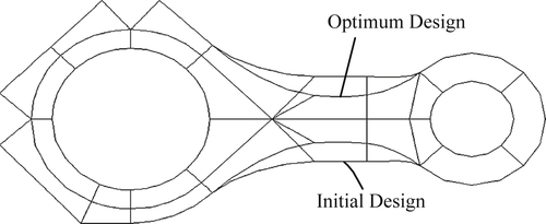
Figure 3.38 shows the design and finite element models at the initial and optimum designs. A reduced optimum weight is obtained by distributing the high stress points along the design boundary Γ1 to Γ6 and making stress constraints active. At the optimum design, the neck region become thinner while stress constraints are not violated.
3.10.3. Shape Optimization of Engine Turbine Blade
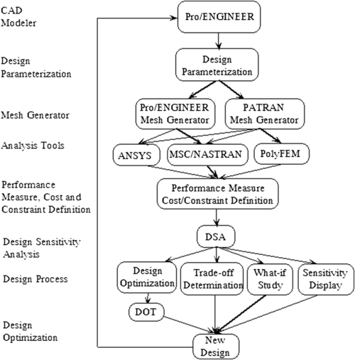
In this case study, we briefly present a shape optimization of a 3-D engine turbine blade using the integrated tool environment shown in Figure 3.39. In this tool set, Pro/ENGINEER is employed to support solid modeling, in which CAD dimensions are defined as design variables for shape optimization. Both Pro/MESH of Pro/ENGINEER and MSC/PATRAN are used to support finite element mesh generation. Commercial FEA codes, including ANSYS, MAS/NASTRA, and PolyFEM (PolyFEM 1994) are integrated to support FEA. Optimization is carried out using DOT.
3.10.3.1. The turbine blade example
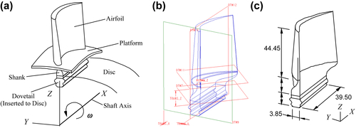
A turbine blade is inserted in a slot of a disc mounted on a rotating shaft, as shown in Figure 3.40 schematically. The blade can be divided into four parts: airfoil, platform, shank, and dovetail. When the turbine is operating, fluid pressure is applied to the surface of the air foil, and an inertia body force is applied to the whole blade structure due to rotation. The inertia body force contributes significantly to the blade structural deformation. To simplify the problem, fluid pressure is, neglected in the finite element and sensitivity analyses. In addition, although the shank sustains a major stress flow from the dovetail to the airfoil due to rotation, the FEA results confirm that the platform does not contribute significantly to blade structural behavior. Thus, the platform is removed in the modeling process. The profile of the airfoil is determined from aerodynamics consideration and is not considered for shape design changes. However, the shape of the shank and the position of the dovetail can be modified to improve structural performance of the blade.
3.10.3.2. CAD and finite element models
The CAD model of the turbine blade shown in Figure 3.40b is created using Pro/ENGINEER. The CAD model is imported into PATRAN for mesh generation. The finite element model shown in Figures 3.34a and b contains 315 3-D 20-node elements (ANSYS STIF95) and 2388 nodes. The material properties are modulus of elasticity E = 2.1 × 10⁵ MPa, Poisson's ratio v = 0.29, and mass density ρ = 7.8 × 10⁻⁶ kg/mm3. For the boundary conditions, displacements of the nodes at two sides of the dovetail are fixed in all directions and a constant angular velocity ω = 1570.8 rad/s (15,000 rpm) is applied to create the inertia body force in the entire blade.
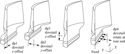
3.10.3.3. Design parameterization for the blade
Four design variables, dp1 to dp4 shown in Figure 3.42, are defined in the model. They are respectively the offset of the dovetail in the X-, Y-, and Z-directions, and rotation of the dovetail about an axis that is parallel to the Z-axis. The four design variables characterize the design changes by repositioning the dovetail. Thus, the dovetail translates with constant cross-sectional shape and straight boundaries, although the shape of the shank changes. Both the shape changes of the shank and translation of the dovetail affect the structural behavior of the blade because the mass is redistributed due to these changes.
3.10.3.4. Design problem definition
The design optimization problem is defined to minimize the volume of the blade and keep stress below a prescribed limit. An optimal design can be achieved by repositioning the dovetail, thereby changing the shape of the shank, which is characterized by the four design variables discussed before. Note that side constraints are defined for the four design variables, as listed in Table 3.9, where design variable dp4 is restricted in the range of −15° to 15° to restrict the dovetail rotation angle outside a ±15° range. The bounds defined for the first design variable ensure the proper alignment of the airfoil in the blade.
At the initial design, structural volume is 15,300 mm3. The von Mises stress at element Gauss points (points for Gauss integration in numerical calculations) of all 315 finite elements are defined as constraints with an upper bound of 4.5 MPa. The 10 finite elements that have stress values over 4.1 MPa in the design iterations are pointed out in Figure 3.41a, and their stress values at initial design are listed in Table 3.10. Also, Z-displacement of nodes at the top surface of the airfoil (77 nodes) and X-displacement of nodes at the front and rear corners of the airfoil (8 nodes) must be less than 5 mm to maintain clearance between the blade and engine casing. These areas are pointed out in Figure 3.41a. Thus, in total, 400 design constraints are defined. As shown in Table 3.10, stress in element 171 is larger than 4.5 MPa; therefore, the initial design is infeasible.
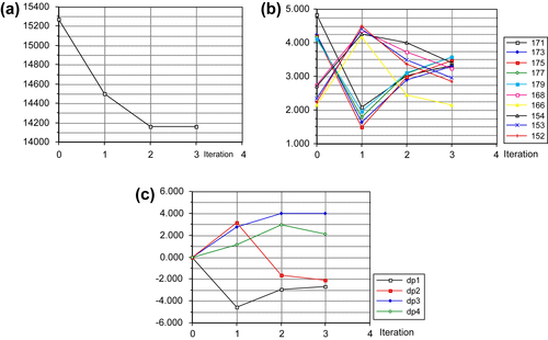
3.10.3.5. Design optimization
An optimal design is found in three design iterations. The optimization history graphs for objective, selected constraints, and design variables are shown in Figures 3.43a, b and c, respectively. The history graphs show that the objective function starts from 15,300 mm3 and reduces to 14,500 mm3 at the first design iteration. During last two iterations, the objective function converges to an optimum criterion defined in the DOT. Note that at the initial design (infeasible), objective function reduction is possible because the design search direction that corrects the constraint violation (stress at element 171) also reduces the objective function value. The objective function value is reduced further until the design reaches a minimum of blade volume 14,150 mm3. Note that the displacement constraints are inactive throughout the design iterations.
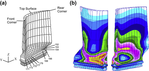
Table 3.10
Selected Gauss Point Stress Measures for the Initial Design
| Element | Stress (MPa) | Upper Bound (MPa) | Status |
| 171 | 4.819 | 4.5 | Violated |
| 173 | 4.226 | 4.5 | Inactive |
| 175 | 4.191 | 4.5 | Inactive |
| 177 | 4.159 | 4.5 | Inactive |
| 179 | 4.102 | 4.5 | Inactive |
| 168 | 2.748 | 4.5 | Inactive |
| 166 | 2.158 | 4.5 | Inactive |
| 154 | 2.712 | 4.5 | Inactive |
| 153 | 2.335 | 4.5 | Inactive |
| 152 | 2.227 | 4.5 | Inactive |
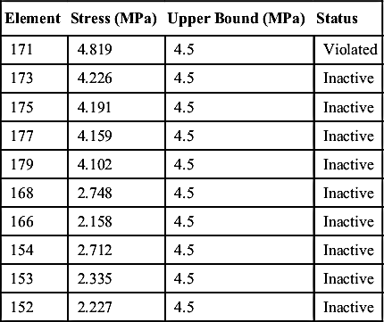
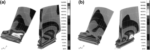
At the optimum, all stresses are below the bound. As shown in Figures 3.44a and b, stress in element 171 is initially greater than the upper bound and is reduced to 3.32 MPa at the optimum design. The highest stress at the optimum is 3.58 MPa, found in element 179. Comparison of stress at element 179 at the optimum to stress at element 171 at initial design shows that stress has been reduced by 25.7%, and the stress in the shank is distributed more evenly at the optimum design, as shown in Figure 3.44b.
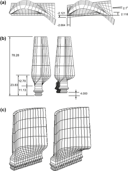
At the optimum, the dovetail rotates 2.1°, which is within the ±15° limit, to adjust stress distribution in the shank. The blade finite element models at the initial and optimum designs are shown in Figure 3.45 for comparison.
..................Content has been hidden....................
You can't read the all page of ebook, please click here login for view all page.