
5.2. Basic Concept
The scalar concept of “optimality” of single-objective optimization problems does not apply directly in the multiobjective setting. To understand the concept and solution techniques, the notion of Pareto optimality has to be introduced. In this section, we start by introducing the criterion space by revisiting the simple MOO example of Example 5.1. We then introduce basic terminologies to facilitate our later discussion. With the basic concept discussed, we revisit the pyramid example to reinforce the concept.
5.2.1. Criterion Space and Design Space
In Example 5.1, we depicted the design space of the MOO problem. We defined its feasible set S, plotted the objective function contours, and identified its Pareto optimal set Sp in design space. Alternatively, a MOO problem can be depicted in the criterion space with axes represented by objective functions. For example, the MOO problem of Example 5.1 can be depicted in its criterion space f1-f2, as shown in Figure 5.2b. Note that the side constraints x1 ≥ 0 and x2 ≥ 0 are translated into the criterion space in this simple example by solving them in terms of f1 and f2:
 (5.4)
(5.4)
The feasible criterion space Z is defined simply as the set of objective function values corresponding to the feasible points in the design space:
![]() (5.5)
(5.5)
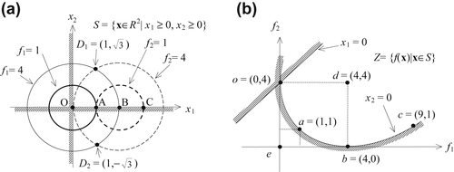
As shown in Figure 5.2a, the points O, A, and B in the design space are mapped into the criterion space at o, a, and b, respectively. The Pareto optimum in the design space Sp = {x ∈ R2| 0 ≤ x1 ≤ 2, x2 = 0} is converted into the curve segment oab in the criterion space, defined as Zp = {f = (f1, f2) ∈ R2| 0 ≤ f1 ≤ 4, 0 ≤ f2 ≤ 4,  = 0}. The curve oab in the criterion space is called the Pareto solution, Pareto optimum, Pareto front, or Pareto set, representing the solutions of the MOO problem. It is clearly shown in the criterion space that the minimum of the objective function f1 is 0 and is located at point o = (0, 4). On the other hand, the minimum of the objective function f2 is 0 and is located at point b = (4, 0). Moreover, an objective function (f1 or f2) cannot be further reduced without increasing the other objective function for any point on the Pareto front. For a point not on the Pareto front, such as point d = (4, 4), it is possible to reduce both objective function values simultaneously by moving the point toward the Pareto front.
A concept related to the feasibility of design points in the design space is that of attainability in criterion space. As discussed in Chapter 3, the feasibility of a design implies that no constraint is violated in the design space. Attainability implies that a point in the criterion space can be related to a point in the design space. It is important to note that each point in the design space can be mapped to the point in the criterion space. However, the reverse may not be true; that is, every point in the criterion space does not necessarily correspond to points or a single point in the design space. For example, point e = (0, 0) in the criterion space does not map back to any point in the design space. Also, point d = (4, 4) in the criterion space maps two points D1 = (1,  ) and D2 = (1, −
 ) in the design space, and D1 ∈ S and D2 ∉ S. We are only interested in the points in the criterion space that are attainable.
5.2.2. Pareto Optimality
The concept in defining solutions for MOO problems is that of Pareto optimality. A point x∗ in the feasible design space S is called Pareto optimal if there is no other point in the set S that reduces at least one objective function without increasing another one. In Example 5.1, the Pareto optimal is x∗ ∈ Sp = {x ∈ R2| 0 ≤ x1 ≤ 2, x2 = 0}. Pareto optimal is defined more precisely as follows.
Definition 1: Pareto Optimal. A point x∗ ∈ S is Pareto optimal iff (i.e., if and only if) ∄ (there does not exist) another point x ∈ S such that fi(x) ≤ fi(x∗) ∀ (for all) i and fi(x) < fi(x∗) for least one i.
To illustrate the above statement, we assume that x∗ = (3, 0) is a Pareto optimal (in fact, it is point C in Figure 5.2a and we know point C is not Pareto optimal). At this point, f1(x∗) = 9 and f2(x∗) = 1. Let us see if f(x) ≤ f(x∗) and fi(x) < fi(x∗) for at least one i are true. We can easily find many points to test the conditions. For example, we pick point A, where x = (1, 0), and f1(x) = f2(x) = 1. Hence, f(x) ≤ f(x∗) with f1(x) = 1 < f1(x∗) = 9. Therefore, from Definition 1, x∗ = (3, 0) is not Pareto optimal. On the other hand, if we pick x∗ = (1, 0) (point A), f1(x∗) = 1 and f2(x∗) = 1. There does not exist any other point where f1 and f2 are less than or equal to those of (1, 0). Hence, x∗ = (1, 0) is a Pareto optimal. In fact, all points in Sp satisfy Definition 1; hence, all are Pareto optimal.
It is important to note that the Pareto optimal set Zp is always on the boundary of the feasible criterion space Z. When there are just two objective functions, as shown in Example 5.1, the minimum points of individual objective functions define the endpoints of the Pareto front (i.e., points o and b in Figure 5.2b), assuming the minima to be unique.
Although the Pareto optimal set is always on the boundary of Z, it is not necessarily defined by the constraints. If the MOO problem of Example 5.1 is redefined as a nonconstrained problem by removing the side constraints x1 ≥ 0, x2 ≥ 0, how do we find the Pareto optimal? In this case, the Pareto optimal is defined by the relationship between the gradients of the objective functions. For cases of two objective functions, the gradients of the objective functions point in opposite directions at all Pareto optimal points (Arora 2012). For the problem in Example 5.1 without side constraints, the Pareto optimal is the line connecting the two centers of the objective function contours, which is unchanged from the constrained problem. From Figure 5.2b, the Pareto optimal can be easily identified on the curve segment oab.
A concept closely related to Pareto optimality is that of weak Pareto optimality. At the weak Pareto optimal points, it is possible to improve some objective functions without penalizing others. A weak Pareto optimal point is defined as follows.
Definition 2: Weak Pareto Optimal. A point x∗ ∈ S is weakly Pareto optimal iff ∄ another point x ∈ S such that fi(x) < fi(x∗) ∀ i.
In another word, a point is weakly Pareto optimal if there is no other point that improves all objective functions simultaneously. However, there may be points that improve some of the objectives while keeping others unchanged.
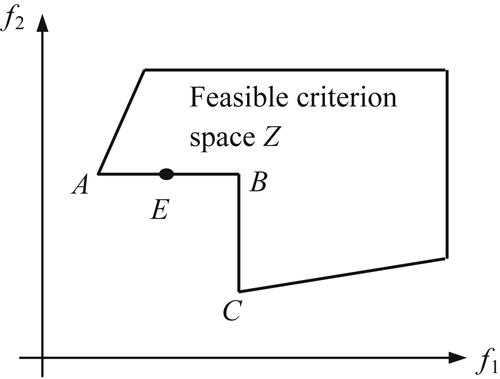
The concept of weak Pareto optimality is illustrated in Figure 5.3. We minimize two objectives f1 and f2. Note that lines AB and BC are the boundary of the feasible criterion space Z and are respectively horizontal and vertical. In this case, all points on line A–B–C are weakly Pareto optimal. However, only points A and C are Pareto optimal.
If we take any point on AB (not including A), such as point E, we cannot find another point x in the feasible criterion space such that f1(x) < f1(xE) and f2(x) < f2(xE); therefore, point E is a weakly Pareto optimal. On the other hand, we can find at least one point x (such as all points between AE) such that f1(x) < f1(xE) and f2(x) = f2(xE); therefore, point E is not Pareto optimal. Similarly, all points on BC (not including C) are weakly Pareto optimal but not Pareto optimal. Pareto optimal is weakly Pareto optimal, but a weakly Pareto optimal is not necessarily Pareto optimal.
Another common concept is that of nondominated and dominated points, which is defined as follows.
Definition 3: Nondominated and Dominated. A vector of objective functions f∗ = f(x∗) ∈ Z is nondominated iff ∄ another vector f ∈ Z such that fi ≤ fi∗ ∀ i and fi < fi∗ for least one i. Otherwise, f∗ is dominated.
Pareto optimality generally refers to both the design and the criterion spaces. In numerical algorithms, the idea of nondomination in the criterion space is often used for a subset of points; one point may be nondominated compared with other points in the subset. A Pareto optimal point has no other point that improves at least one objective without detriment to another; that is, it is nondominated.
A unique point, called utopia point or ideal point, in the criterion space is defined as follows.
Definition 4: Utopia Point. A point fo in the criterion space is called the utopia point if  = min{fi(x) |x ∈ S}, i = 1 to q, and q is the number of the objective functions.
The utopia point is obtained by minimizing each objective function without regard for other objective functions. Each minimization yields a design point in the design space and the corresponding value for the objective function. As shown in Figure 5.2b, point e is the utopia point of Example 5.1.
In general, it is rare that each minimization will end up at the same point in the design space. That is, one design point cannot simultaneously minimize all of the objective functions. Thus, the utopia point exists only in the criterion space and, in general, it is not attainable, such as the utopia point e in Figure 5.2b.
The next best thing to a utopia point is a Pareto solution that is as close as possible to the utopia point. Such a solution is called a compromise solution, for example, point a in Figure 5.2b. The term closeness can be defined in several different ways. Usually, it implies that one minimizes the Euclidean distance D(x) from the utopia point in the criterion space, which is defined as follows:
 (5.6)
(5.6)
where represents a component of the utopia point in the criterion space. Compromise solutions are Pareto optimal.
5.2.3. Generation of Pareto Optimal Set
For a simple problem such as Example 5.1, we can easily solve it by translating the problem from design space to criterion space and identifying its Pareto optimal set in the criterion space as Zp = {f = (f1, f2) ∈ R2| 0 ≤ f1 ≤ 4, 0 ≤ f2 ≤ 4, = 0}. The Pareto optimal set can also be translated back to its design space Sp = {x ∈ R2| 0 ≤ x1 ≤ 2, x2 = 0}. For problems just a bit more complicated, such as the pyramid design, none of the above is possible. So, how do we solve MOO problems in general?
We first use a brute-force approach—the generative method similar to that discussed in Chapter 3—to solve for the pyramid problem. We will then make a few comments before moving into the next section for the discussion of general solution techniques.
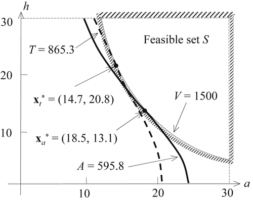
Recall the problem definition of the pyramid problem in Eq. 5.2. The feasible set of the problem is defined in its design space (in this case, the a-h plane) as
![]() (5.7)
(5.7)
The feasible set S is graphed in Figure 5.4, with optimal points  = (14.7, 20.8) and
  = (18.5, 13.1) for objective functions T and A, respectively. Note that the optimal points and are obtained by solving the two respective single-objective problems using MATLAB (Script 1 in Appendix A).
Translating this simple problem from design space to its criterion space is not straightforward. In fact, it is very difficult, if not entirely impossible, to write the design variables a and h as functions of objective functions A and T analytically. Therefore, we use the generative method to graph feasible and infeasible solutions in criterion space.
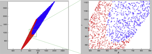
We first generate 1,000,000 random points for a and h, respectively. We then calculate the numerical values of the two objective functions A and T for each point (a, h). In the meantime, we calculate volume V. If V is greater or equal to 1500, the design represented in the point (a, h) is feasible; otherwise, it is infeasible. We store feasible and infeasible points separately and graph them on the criterion space in different colors. The points at the junction of the areas of different colors are the boundary of the feasible criterion space Z. Once the feasible criterion space is identified, we locate the minimum points of functions A and T and identify the Pareto front. The MATLAB script that graphs the criterion space and Pareto front shown in Figure 5.5 can be found in Appendix A (Script 2). The MATLAB script also found that the minima of A and T are, respectively, 594.8 and 865.5. The minimum A occurs at a = 18.63 and h = 12.97, which is very close to the found earlier (see Figure 5.4). The minimum T occurs at a = 14.56 and h = 21.23, which is again very close to .
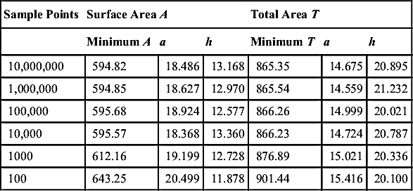
In fact, we ran six cases with sample points ranging from 100 to 10,000,000, as shown in Table 5.1. The results show that for sample points more than 10,000, the results do not vary significantly. However, if we graph the criterion space with a sample size of 10,000, the boundary of the feasible criterion set, hence the Pareto front, cannot be clearly identified (see Figure 5.6).
Although the generative method is simple, it works well only for simple problems, such as the pyramid example. In general, engineering design problems involve significant computation efforts for function evaluations, and it is impractical to find Pareto front using the generative method in general. On the other hand, do we really need to solve for an entire set of the Pareto front in order to make adequate design decisions? Instead of the generative method, are there plausible methods that are practical for support of engineering design involving multiple objectives?
We discuss solution techniques for multiobjective optimization problems in the next section. Note that a key characteristic of MOO solution techniques is the nature of the solutions that they provide. Some methods always yield Pareto optimal solutions but may skip certain points in the Pareto optimal set; that is, they may not be able to yield all or most of the Pareto optimal points. Other methods are able to capture most points in the Pareto optimal set, but they may also provide non-Pareto optimal points. In any case, the primary goal of solving a multiobjective optimization problem is to support the designer to make adequate design decision, which may involve the designer's preferences in ordering or setting the relative importance of individual objective functions. A designer may articulate these preferences before solving the MOO problem or wait until sufficient solutions become available and then set the preferences. In some cases, a designer may not have any preferences at all. Different solution techniques are suitable for the respective situations.
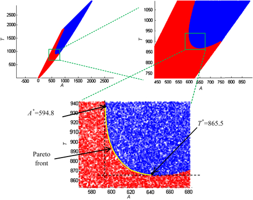
Table 5.1
Cases of the Pyramid Example with Different Sample Sizes Ranging from 100 to 10,000,000
| Sample Points | Surface Area A | Total Area T | ||||
| Minimum A | a | h | Minimum T | a | h | |
| 10,000,000 | 594.82 | 18.486 | 13.168 | 865.35 | 14.675 | 20.895 |
| 1,000,000 | 594.85 | 18.627 | 12.970 | 865.54 | 14.559 | 21.232 |
| 100,000 | 595.68 | 18.924 | 12.577 | 866.26 | 14.999 | 20.021 |
| 10,000 | 595.57 | 18.368 | 13.360 | 866.23 | 14.724 | 20.787 |
| 1000 | 612.16 | 19.199 | 12.728 | 876.89 | 15.021 | 20.336 |
| 100 | 643.25 | 20.499 | 11.878 | 901.44 | 15.416 | 20.100 |
..................Content has been hidden....................
You can't read the all page of ebook, please click here login for view all page.