
3.7. Non-Gradient Approach
Unlike the gradient-based approach, the non-gradient approach uses only the function values in the search process, without the need for gradient information. The algorithms developed in this approach are very general and can be applied to all kinds of problems—discrete, continuous, or nondifferentiable functions. In addition, the methods determine global optimal solutions as opposed to the local optimal determined by a gradient-based approach. Although the non-gradient approach does not require the use of gradients of objective or constraint functions, the solution techniques require a large amount of function evaluations. For large-scale problems that require significant computing time for function evaluations, the non-gradient approach is too expensive to use. Furthermore, there is no guarantee that a global optimum can be obtained. The computation issue may be overcome to some extent by the use of parallel computing or supercomputers. The issue of global optimal solution may be overcome to some extent by allowing the algorithm to run longer.
In this section, we discuss two popular and representative algorithms of the non-gradient approach: the genetic algorithm (GA) and simulated annealing (SA). We introduce concepts and solution process for the algorithms to provide readers with a basic understanding of these methods.
3.7.1. Genetic Algorithms
Recall that the optimization problem considered is defined as
![]() (3.87)
(3.87)
where S is the set of feasible designs defined by equality and inequality constraints. For unconstrained problems, S is the entire design space. Note that to use a genetic algorithm, the constrained problem is often converted to an unconstrained problem using, for example, the penalty method discussed in Section 3.6.6.
3.7.1.1. Basic concepts
A genetic algorithm starts with a set of designs or candidate solutions to a given optimization problem and moves toward the optimal solution by applying the mechanism mimicking evolution principle in nature—that is, survival of the fittest. The set of candidate solutions is called a population. A candidate solution in a population is called individual, creature, or phenotype. Each candidate solution has a set of properties represented in its chromosomes (or genotype) that can be mutated and altered. Traditionally, candidate solutions are represented in binary strings of 0 and 1, but other encodings are also possible. The evolution usually starts from a population of randomly generated individuals. The solution process is iterative, with the population in each iteration called a generation. The size of the population in each generation is unchanged. In each generation, the fitness of every individual in the population is evaluated; the fitness is usually the value of the objective (or pseudo-objective converted from a constrained problem) function in the optimization problem being solved. The better fit individuals are stochastically selected from the current population, and each individual's genome is modified (recombined and possibly randomly mutated) to form a new generation. Because better fit members of the set are used to create new designs, the successive generations have a higher probability of having designs with better fitness values. The new generation of candidate solutions is then used in the next iteration of the algorithm. Commonly, the algorithm terminates when either a maximum number of generations has been reached or a satisfactory fitness level has been achieved for the population.
3.7.1.2. Design representation
In a genetic algorithm, an individual (or a design point) consists of a chromosome and a fitness function.
The chromosome represents a design point, which contains values for all the design variables of the design problem. The gene represents the value of a particular design variable. The simplest algorithm represents each chromosome as a bit string. Typically, an encoding scheme is prescribed, in which numeric parameters can be represented by integers, although it is possible to use floating point representations as well. The basic algorithm performs crossover and mutation at the bit level. For example, we assume an optimization problem of three design variables: x = [x1, x2, x3]T. We use a string length of 4 (or 4 bits) for each design variable, in which 24 = 16 discrete values can be represented. If, at the current design, the design variables are x1 = 4, x2 = 7, and x3 = 1, the chromosome length is C = 12:
With a method to represent a design point defined, the first population consisting of Np design points (or candidate solutions) needs to be created. Np is the size of the population. This means that Np strings need to be created. In some cases, the designer already knows some good usable designs for the system. These can be used as seed designs to generate the required number of designs for the population using some random process. Otherwise, the initial population can be generated randomly via the use of a random number generator. Back to the example of three design variables x = [x1, x2, x3]T, Np number of random variables of C = 12 digits can be generated. Let us say one of them is 803590043721. A rule can be set to convert the random number to a string of 0 and 1. The rule can be, for example, converting any value between zero and four to “0,” and between five and nine to “1.” Following this rule, the random number is converted to a string 100110000100, representing a design point of x1 = 9 (decoded from string: 1001), x2 = 8 (string: 1000), and x3 = 4 (string: 0100).
Once a design point is created, its fitness function is evaluated. The fitness function defines the relative importance of a design. A higher fitness value implies a better design. The fitness function may be defined in several different ways. One commonly employed fitness function is
![]() (3.88)
(3.88)
where fmax is the maximum objective function value obtained by evaluating at each design point of the current population, and fi and Fi are the objective function value and fitness function value of the ith design point, respectively.
3.7.1.3. Selection
The basic idea of a genetic algorithm is to generate a new set of designs (population) from the current set such that the average fitness of the population is improved, which is called a reproduction or selection process. Parents are selected according to their fitness; for example, each individual is selected with a probability proportional to its fitness value, say 50%, meaning that only half of the population with the best fitness functions is selected as parents to breed the next generation by undergoing genetic operations, to be discussed next. By doing so, weak solutions are eliminated and better solutions survive to form the next generation. The process is continued until a stopping criterion is satisfied or the number of iterations exceeds a specified limit.
3.7.1.4. Reproduction process and genetic operations
There are many different strategies to implement the reproduction process; usually a new population (children) is created by applying recombination and mutation to the selected individuals (parents). Recombination creates one or two new individuals by swapping (crossing over) the genome of a parent with another. A recombined individual is then mutated by changing a single element (genome) to create a new individual. Crossover and mutation are the two major genetic operations commonly employed in the genetic algorithms.
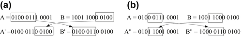
Crossover is the process of combining or mixing two different designs (chromosomes) into the population. Although there are many methods for performing crossover, the most common ones are the one-cut-point and two-cut-point methods. A cut point is a position on the genetic string. In the one-cut-point method, a position on the string is randomly selected that marks the point at which two parent design points (chromosomes) split. The resulting four halves are then exchanged to produce new designs (children). For example, string A = 0100 0111 0001, representing design xA = (4, 7, 1) and string B = 1001 1000 0100 representing xB = (9, 8, 4) are two design points of the current generation. If the cut point is randomly chosen at the seventh digit, as shown in Figure 3.18a, the new strings become A′ = 0100 0110 0100, in which the last five digits were replaced by those of string B, and B′ = 0100 0110 0100, in which the first seven digits were replaced by those of string A. As a result, two new designs are created for the next generation, i.e., xA′ = (4, 6, 4) and xB′ = (4, 6, 4). These two new design points (children) xA′ and xB′ are identical, which is less desirable.
Similarly, the two-cut-point method is illustrated in Figure 3.18b, in which the two cut points are chosen as 3 and 7, respectively. The two new strings become A″ = 0101 1001 0001, in which the third to sixth digits were replaced by those of string B, and similarly B″ = 1000 0110 0100. As a result, two new designs are created for the next generation: xA″ = (5, 9, 1) and xB′ = (8, 3, 4).
Selecting how many or what percentage of chromosomes to crossover, and at what points the crossover operation occurs, is part of the heuristic nature of genetic algorithms. There are many different approaches, and most are based on random selections.
Mutation is another important operator that safeguards the process from a complete premature loss of valuable genetic material during crossover. In terms of a binary string, this step corresponds to the selection of a few members of the population, determining a location on the strings at random, and switching the 0 to 1 or vice versa.
Similar to the crossover operator, the number of members selected for mutation is based on heuristics, and the selection of location on the string for mutation is based on a random process.
Let us select a design point as “1000 1110 1001” and select the 7th digit to mutate. The mutation operation involves replacing the current value of 1 at the seventh location with 0 as “1000 1100 1001.”
For example, string C = 1110 0111 0101 represents design xC = (14, 7, 5). If we choose the seventh digit to mutate, the new strings become C′ = 1110 0101 0101. As a result, the new design is created for the next generation as xC′ = (14, 5, 5).
In numerical implementation, not all individuals in a population go through crossovers and mutations. Too many crossovers can result in a poorer performance of the algorithm because it may produce designs that are far away from the mating designs (designs of higher fitness value). The mutation, on the other hand, changes designs in the neighborhood of the current design; therefore, a larger amount of mutation may be allowed. Note also that the population size needs to be set to a reasonable number for each problem. It may be heuristically related to the number of design variables and the number of all possible designs determined by the number of allowable discrete values for each variable. Key parameters, such as the number of crossovers and mutations, can be adjusted to fine-tune the performance of the algorithm. In general, the probability of crossover being applied is typically less than 0.1, and probability of mutation is between 0.6 and 0.9.
3.7.1.5. Solution process
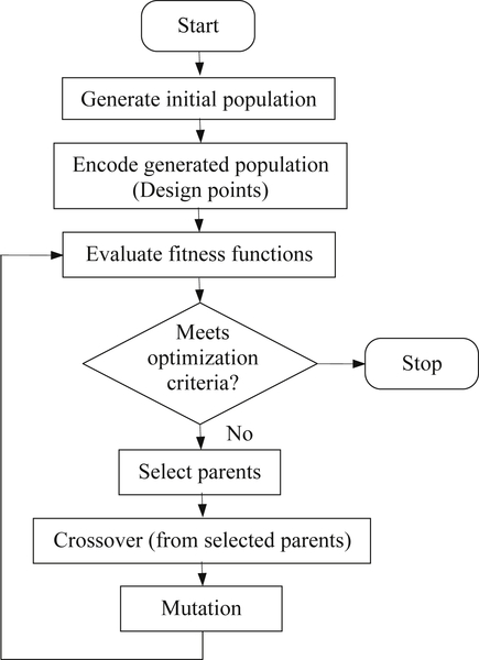
A typical solution process of a genetic algorithm is illustrated in Figure 3.19. The initial population is usually generated randomly in accordance with the encoding scheme. Once a population is created, fitness function is assigned or evaluated to individuals in the population, for example, using Eq. 3.88. Parents are then selected according to their fitness. Genetic operations, including crossover and mutation, are performed to create children. The fitness of the new population is evaluated and the process is repeated until stopping criteria are met. The stopping criteria include (a) the improvement for the best objective (or pseudo-objective) function value is less than a small tolerance ε0 for the last n consecutive iterations (n is chosen by the users), or (b) if the number of iterations exceeds a specified value.
3.7.2. Simulated Annealing
Simulated annealing is a stochastic approach that locates a good approximation to the global minimum of a function. The main advantage of SA is that it can be applied to broad range of problems regardless of the conditions of differentiability, continuity, and convexity that are normally required in conventional optimization methods. Given a long enough time to run, an algorithm based on this concept finds global minima for an optimization problem that consists of continuous, discrete, or integer variables with linear or nonlinear functions that may not be differentiable.
The name of the approach comes from the annealing process in metallurgy. This process involves heating and controlled cooling of a material to increase the size of its crystals and reduce their defects. Simulated annealing emulates the physical process of annealing and was originally proposed in the domain of statistical mechanics as a means of modeling the natural process of solidification and formation of crystals. During the cooling process, it is assumed that thermal equilibrium (or quasi-equilibrium) conditions are maintained. The cooling process ends when the material reaches a state of minimum energy, which, in principle, corresponds with a perfect crystal.
3.7.2.1. Basic concept
The basic idea for implementation of this analogy to the annealing process is to generate random points in the neighborhood of the current best design point and evaluate the problem functions there. If the objective function value is smaller than its current best value, the design point is accepted and the best function value is updated. If the function value is higher than the best value known thus far, the point is sometimes accepted and sometimes rejected. Nonimproving (inferior) solutions are accepted in hope of escaping an local optimum in search of the global optimum. The probability of accepting non-improving solutions depends on a “temperature” parameter, which is typically nonincreasing with each iteration. One commonly employed acceptance criterion is stated as
 (3.89)
where P(x′) is the probability of accepting the new design x′ randomly generated in the neighborhood of x, x is the current best point (of iteration k), and T k is the temperature parameter at the kth iteration, such that
![]() (3.90)
(3.90)
where temperature parameter T k is positive, and is decreasing gradually to zero when the number of iterations k reaches a prescribed level. In implementation, k is not approaching infinite but a sufficiently large number. Also, as shown in Eq. 3.89, the probability of accepting an inferior design depends on the temperature parameter T k. At earlier iterations, T k is relative large; hence, the probability of accepting an inferior design is higher, providing a means to escape the local minimum by allowing so-called hill-climbing moves. As the temperature parameter T k is decreased in later iterations, hill-climbing moves occur less frequently, and the algorithm offers a better chance to converge to a global optimal. Hill-climbing is one of the key features of the simulated annealing method.
As shown in Eq. 3.90, the algorithm demands a gradual reduction of the temperature as the simulation proceeds. The algorithm starts initially with T k set to a high value, and then it is decreased at each step following some annealing schedule—which may be specified by the user, or set by a parameter, such as
![]() (3.91)
(3.91)
where is T k+1 the temperature for the next iteration k + 1.
3.7.2.2. Solution process
We start the solution process by choosing an initial temperature T 0 and a feasible trial point x0. Compute objective function f(x0). Select an integer L (which sets a limit on the number of iterations), and a parameter r < 1.
At the kth iteration, we then generate a new point x′ randomly in a neighborhood of the current point xk. If the point is infeasible, generate another random point until feasibility is satisfied. Check if the new point x′ is acceptable. If f(x′) < f(xk), then accept x′ as the new best point, set xk+1 = x′, and continue the iteration. If f(x′) ≥ f(xk), then calculate P(x′) using Eq. 3.89. In the meantime, we generate a random number z uniformly distributed in [0, 1]. If P(x′) > z, then accept x′ as the new best point and set xk+1 = x′ to continue the iteration. If not, we generate another new point x″ randomly, and repeat the same steps until a new best point is found. We repeat the iteration, until k reaches the prescribed maximum number of iterations L.
..................Content has been hidden....................
You can't read the all page of ebook, please click here login for view all page.