5.6. Advanced Topics

Search in book...
Toggle Font Controls
Create new playlist

Name your new playlist

Playlist description (optional)
Sign In

Email address

Password

Forgot Password?

or

Continue with Facebook

Continue with Google
Sign Up

Full Name

Email address

Confirm Email Address

Password

or

Continue with Facebook

Continue with Google

5.6. Advanced Topics

Before closing out this chapter, we include two advanced topics that are relevant to design optimization. The first topic is reliability-based design optimization (RBDO), which incorporates variations in physical parameters and design variables into design optimization, leading to design with less probability of failure. Second, we introduce a case of design optimization that takes product cost, including manufacturing, as an objective function. This case represents a more realistic design optimization problem that leads to less expensive designs.

5.6.1. Reliability-Based Design Optimization

In Chapter 5 of Chang (2013a), we discussed reliability analysis. We introduced the concept of failure modes associated with certain critical product performance. We incorporated the variability (or uncertainty) of physical parameters or a manufacturing process that affects the performance (hence, failure modes) of the product to estimate a failure probability. We used a beam example for illustration, in which the failure probability of a stress failure mode predicts the percentage of the incidents when the maximum stress of the beam exceeds its material yield strength. The result offered by the reliability analysis is far more precise and effective than that of the safety factor approach.

In this subsection, we move one step further to discuss design optimization by incorporating failure modes (and failure probabilities) into optimization problem formulation. We first briefly review the basics of the reliability analysis, in particular, the most probable point (MPP) search for failure probability estimates. We then formulate the mathematic equations for a standard RBDO and its solution technique, and we present a sample case to illustrate the topic of RBDO using a tracked-vehicle roadarm example. Readers are encouraged to review Chapter 5 of Chang (2013a) to refresh the concept and numerical computations involved in the reliability analysis before reading further.

5.6.1.1. Failure probability

The probability of failure P_f of a product with a failure mode g(X) ≤ 0 is defined as

$P_{f} = P (M \leq 0) = P (g (X) \leq 0) = \int_{g (x) \leq 0} f_{X} (x) d x$

(5.35)

where f_X(x) is the joint probability density function (PDF), X is a vector of random variables, and the function g(x) = 0 is called the limit state function. Note that realization of X = [X₁,X₂,…,X_n]^T is denoted as x = [x₁,x₂,…,x_n]^T, which is a point in the n-dimensional space.

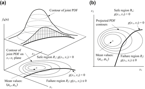
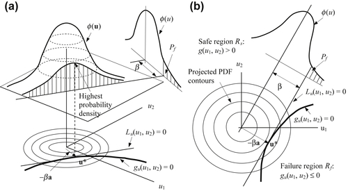
The probability integration in Eq. 5.35 is visualized for a two-dimensional case in Figure 5.30a, which shows the joint PDF f_X(x) and its contour projected onto the x₁-x₂ plane. All the points on the projected contours have the same values of f_X(x) or the same probability density. The limit state function g(x) = 0 is also shown. The failure probability P_f is the volume underneath the surface of the joint PDF f_X(x) in the failure region g(x) ≤ 0. To show the integration more clearly, the contours of the joint PDF f_X(x) and the limit state function g(x) = 0 are plotted on the x₁-x₂ plane, as shown in Figure 5.30b.

The direct evaluation of the probability integration of Eq. 5.35 is very difficult if not impossible. A number of methods have been developed. Monte Carlo simulation is simple and easy to implement. However, this brute-force approach requires tens of thousands analyses or more, which is impractical for engineering problems that often require significant computational effort. One of the widely employed methods to alleviate the computational issue to some extent, while still offering a sufficiently accurate estimate on the failure probability, is the first-order reliability method (FORM). This method aims at providing an acceptable estimate for the integral form of the failure probability P_f defined in Eq. 5.35, which can be achieved by two important steps. The first step involves the simplification of the joint probability density function f_X(x). The simplification is accomplished by transforming a given joint probability density function, which may be multidimensional, to a standard normal distribution function of independent random variables of the same dimensions. The second step approximates the limit state function g(x) = 0 by a Taylor's series expansion and keeps up to the first-order terms for approximation. Note that if both linear and quadratic terms are included in the calculation, the method is called the second-order reliability method (SORM).

FIGURE 5.30 Probability integration illustrated using a two-dimensional example. (a) Isometric view. (b) Projected view on the x₁-x₂ plane.

The space that contains the given set of random variables X = [X₁,X₂,…,X_n]^T is called the X-space. These random variables are transformed to a standard normal space (U-space), where the transformed random variables U = [U₁,U₂,…,U_n]^T follow the standard normal distribution (i.e., with mean value μ = 0 and standard deviation σ = 1). Such a transformation is carried out based on the condition that the cumulative density functions (CDFs) of the random variables remain the same before and after transformation; that is,

$F_{X_{i}} (x_{i}) = Φ (u_{i})$

(5.36)

Here,

$Φ (\cdot)$

is the CDF of the standard normal distribution. The transformation can be written as

$u_{i} = Φ^{- 1} (F_{X_{i}} (x_{i}))$

(5.37a)

Hence, the transformed random variable U_i can be written as

$U_{i} = Φ^{- 1} (F_{X_{i}} (X_{i}))$

(5.37b)

If the random variables X_i are independent and normally distributed—that is,

$F_{X_{i}} (x_{i}) = Φ (\frac{x_{i} - μ_{i}}{σ_{i}})$

— the transformation, as illustrated in Figure 5.31, can be obtained as

$u_{i} = Φ^{- 1} (Φ (\frac{x_{i} - μ_{i}}{σ_{i}})) = \frac{x_{i} - μ_{i}}{σ_{i}}$

(5.38)

Hence,

$x_{i} = μ_{i} + σ_{i} u_{i}$

(5.39)

Note that, as shown in Figure 5.31c, the projected contours of the transformed PDF on the u₁-u₂ plane are circles centered at the origin.

The limit state function is also transformed into the U-space, as

$g (x) = g_{u} (u) = 0$

(5.40)

FIGURE 5.31 Transformation of random variables from X to U, illustrated using a two-dimensional example. (a) PDF and projected contours in X-space. (b) Standard normal distribution in U-space. (c) Projected view on the u₁-u₂ plane.

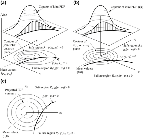
The transformed limit state function separates the U-space into safe and failure regions, as illustrated in Figure 5.31b and c. After the transformation, the probability integration of Eq. 5.35 becomes

$P_{f} = P (g_{u} (u) \leq 0) = \int_{g_{u} (u) \leq 0} ϕ (u) d u$

(5.41)

Because all of the random variables U are independent, the joint PDF is the product of the individual PDFs of standard normal distribution:

$ϕ (u) = \prod_{i = 1}^{n} \frac{1}{\sqrt{2 π}} e^{- \frac{1}{2} u_{i}^{2}}$

(5.42)

Therefore, the probability integration becomes

$P_{f} = \iint \dots \int_{g_{u} (u) \leq 0} \prod_{i = 1}^{n} \frac{1}{\sqrt{2 π}} e^{- \frac{1}{2} u_{i}^{2}} d u_{1} d u_{2} \dots d u_{n}$

(5.43)

Although it is obvious that Eq. 5.43 is relatively easier to calculate than Eq. 5.35, calculating Eq. 5.43 is still difficult because the limit state function g_u(u) is in general a nonlinear function of variables u.

If the nonlinearity of the limit state function is not too severe, the integration of Eq. 5.43 can be approximated by

$P_{f} \approx \int_{- \infty}^{- β} \frac{1}{\sqrt{2 π}} e^{- \frac{1}{2} u^{2}} d u = Φ (- β)$

(5.44)

where Φ is the standard normal distribution function of a single dimension, and β is the shortest distance between the origin and the point on the limit state function g_u(u) = 0. This point is depicted as u∗ in Figure 5.32 and is called the β-point, design point, or the most probable point. The β value is called reliability index.

FIGURE 5.32 Approximation of failure probability integration, illustrated using a two-dimensional example. (a) PDF and projected contours in the U-space. (b) Projected view on the u₁-u₂ plane.

As illustrated in Figure 5.32a, the line that connects the origin and the MPP must be perpendicular to the tangent line L_u(u₁,u₂) = 0 at the MPP. Because the joint PDF ϕ(u) of the multidimension is axisymmetric, its projection on the plane that is normal to the tangent line is nothing but a probability density function of the standard normal distribution ϕ(u) of a single dimension. The probability integration of Eq. 5.35 can then be approximated by

$Φ (- β)$

, as stated in Eq. 5.44.

As discussed above, the key idea in calculating the failure probability using FORM or SORM is to locate the MPP in the U-space. Many numerical approaches have been developed for the MPP search. These methods can be categorized in two major categories: the reliability index approach (RIA) and the performance measure approach (PMA). The reliability index approach employs a forward reliability analysis algorithm that computes failure probability for a prescribed performance level in the limit state function. The performance measure approach employs an inverse reliability analysis algorithm that computes response level for a prescribed failure probability. We briefly state both approaches. For more details, readers are referred to Chang (2013a).

The problem for MPP search using RIA can be formulated as follows:

$\begin{matrix} Minimize : & ‖ u ‖ \\ Subject to : & g_{u} (u) = 0 \end{matrix}$

(5.45)

in which the MPP is identified by searching a point on the limit state function

$g_{u} (u) = 0$

, where the distance between the point to the origin of the U-space is minimum. Again, the distance β is called the reliability index, hence the name of this approach. Note that in Eq. 5.45, the performance level of the limit state function is prescribed. In this case, MPP can only be searched for the performance level prescribed. Once the MPP is found, the distance β (reliability index) can be used to approximate the failure probability as P_f = Φ(−β).

The performance measure approach, on the other hand, is given a target reliability index β (or failure probability P_f, and then

$β = Φ^{- 1} (P_{f})$

). Thereafter, we search for MPP by bringing the function g_u(u) closer to

$g_{u} (u) = 0$

, in which the target performance level is achieved. The concept of PMA is illustrated in Figure 5.33 using a two-dimensional example. The required reliability index β is shown as a circle centered at the origin of the u₁-u₂ plane with radius β. Depending on the u value entered for the MPP search, the limit state function g_u(u) usually is nonzero. If the u value entered is in the safe region, then g_u(u) > 0. On the other hand, if u is in the failure region, g_u(u) < 0. The MPP search becomes finding u that brings the limit state function g_u(u) to g_u(u) = 0. Therefore, the problem for MPP search using PMA can be formulated as follows:

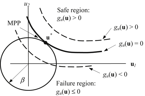
FIGURE 5.33 MPP search using the performance measure approach.

$\begin{matrix} Minimize : & | g_{u} (u) | \\ Subject to : & β = ‖ u ‖ \end{matrix}$

(5.46)

in which the reliability index

$β = Φ^{- 1} (P_{f})$

, and P_f is the required failure probability. Also, in Eq. 5.46, the limit state function g_u(u) can be rewritten as

$g_{u} (u) = {g^{t}}^{'} (u) - g^{t}$

(5.47)

where g^t(u) is the performance measure corresponding to the failure mode, and g^t is the target performance level.

Next, we formulate the standard reliability-based design optimization problems, in which we assume the RIA for the MPP search.

5.6.1.2. RBDO problem formulation

The classical design optimization problem based on deterministic analysis is typically formulated as a nonlinear constrained optimization problem, as discussed in Chapter 3. Similarly, the RBDO problem can also be formulated as a nonlinear constrained optimization problem where reliability measures are included as constraint functions. Probabilistic constraints in RBDO ensure a more evenly distributed failure probability in the component of a product. In general, the RBDO model contains two types of design variables: distributional design variable θ and conventional deterministic design variable b.

Let θ = [θ₁,θ₂,...,θ_n1]^T and b = [b₁,b₂,...,b_n2]^T be the distributional and deterministic design variable vectors of dimensions n₁ and n₂, respectively. The RBDO problem can be formulated as follows:

$Minimize : f (θ, b)$

(5.48a)

$Subject to : P_{f_{i}} = P (g_{i} (θ, b) \leq 0) - P_{i}^{u} \leq 0, i = 1, m$

(5.48b)

$θ_{j}^{ℓ} \leq θ_{j} \leq θ_{j}^{u}, j = 1, n_{1}$

(5.48c)

$b_{k}^{ℓ} \leq b_{k} \leq b_{k}^{u}, k = 1, n_{2}$

(5.48d)

where f(θ, b) is the objective function, P(•) denotes the probability of the event (•), and P_i^u is the required upper bound of the probability of failure for the ith constraint function

$P_{f_{i}}$

. In Eqs (5.48c) and (5.48d),

$θ_{j}^{ℓ}$

and

$θ_{j}^{u}$

, and

$b_{k}^{ℓ}$

and

$b_{k}^{u}$

, are the lower and upper bounds of the jth distributional and kth deterministic design variables, respectively.

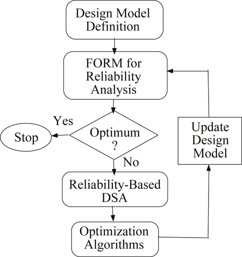
The reliability constraints defined in Eq. 5.48b are assumed to be independent and thus no correlation exists. As mentioned, it is almost impossible to calculate the probability of failure

$P_{f_{i}}$

in Eq. 5.48b by a multiple integration for general design applications. Consequently, the FORM or other more efficient reliability analysis methods are employed. The computational flow of RBDO using the FORM is illustrated in Figure 5.34. Note that at each design iteration, the FORM needs to be carried out several times for individual failure functions. As formulated in Eq. 5.45, each FORM is equivalent to a deterministic optimization, which is very computationally demanding. This is the reason why RBDO is mostly limited to academic problems. Furthermore, the first-order derivative of the failure probability with respect to both distributional and deterministic design variables must be computed to support gradient-based RBDO.

FIGURE 5.34 Computation flow for gradient-based RBDO.

5.6.1.2.1. Reliability-based design sensitivity analysis

The sensitivity of the failure probability includes two parts: the sensitivity of the failure probability with respect to the distributional parameters θ of random variables (e.g., mean value, standard deviation), and the sensitivity of the failure probability with respect to the deterministic design variables b.

The derivative of the estimated failure probability P_f obtained using the FORM with respect to a design variable η, which can be either θ_j or b_k, is

$\frac{\partial P_{f}}{\partial η} = \frac{\partial Φ (- β)}{\partial η} = \frac{\partial Φ (- β)}{\partial β} \frac{\partial β}{\partial η} = - Φ (- β) \frac{\partial β}{\partial η}$

(5.49)

where Φ is the standard normal density function. Therefore, to compute the sensitivity of the failure probability P_f, ∂β/∂η must be computed as

$\frac{\partial β}{\partial η} = \frac{\partial {(U^{*^{T}} U^{*})}^{1 / 2}}{\partial η} = \frac{1}{β} U^{*^{T}} \frac{\partial U^{*}}{\partial η}$

(5.50)

where U^∗ is the MPP found in the U-space.

The sensitivity of the reliability index with respect to a distributional design variable θ_j can be obtained by substituting η = θ_j and U^∗ = T(X^∗, θ) in Eq. 5.50 as

$\frac{\partial β}{\partial θ_{j}} = \frac{1}{β} U^{*^{T}} (\frac{\partial T (X^{*}, θ)}{\partial θ_{j}} + \frac{\partial T (X^{*}, θ)}{\partial X^{*}} \frac{\partial X^{*}}{\partial θ_{j}}) = \frac{1}{β} U^{*^{T}} \frac{\partial T (X^{*}, θ)}{\partial θ_{j}}$

(5.51)

For the normally distributed random variables, where T can be explicitly written as a transformation function of θ, Eq. 5.51 can be calculated analytically. For the non-normally distributed random variables, the transformation T cannot be obtained explicitly. In such a case, the finite difference method can be used to approximate the derivative of T with respect to θ_j.

As discussed, the reliability index β is the distance between the origin and the MPP in the U-space. The MPP vector U^∗ on the failure surface can be written as

$U^{*} = - β \frac{\nabla g (U^{*}, b)}{| \nabla g (U^{*}, b) |}$

(5.52)

in which, ∇g(U^∗,b) is the gradient of the failure function at the MPP:

$\nabla g (U^{*}, b) = \frac{\partial g (U^{*}, b)}{\partial U}$

(5.53)

From Eq. 5.52, the MPP vector U^∗ is also a function of b because the failure function g depends on the deterministic design variables b. Substituting Eq. 5.52 into Eq. 5.50 yields

$\frac{\partial β}{\partial b} = - \frac{1}{| \nabla g (U^{*}, b) |} \frac{\partial g^{T} (U^{*}, b)}{\partial U} \frac{\partial U^{*}}{\partial b}$

(5.54)

By taking the derivative of g(U^∗, b) = 0 with respect to b,

$\frac{\partial g^{T} (U^{*}, b)}{\partial U} \frac{\partial U^{*}}{\partial b} + \frac{\partial g (U^{*}, b)}{\partial b} = 0$

(5.55)

Substituting Eq. 5.55 into Eq. 5.54 yields

$\frac{\partial β}{\partial b} = \frac{1}{| \nabla g (U^{*}, b) |} \frac{\partial g^{T} (U^{*}, b)}{\partial b}$

(5.56)

Note that evaluation of Eq. 5.56 needs only the first-order derivative of the failure function with respect to deterministic design variables.

To avoid the prohibitively expensive computational efforts required for a large number of reliability analyses during a batch-mode RBDO for design optimization, a mixed-design approach (Yu et al. 1997) that includes deterministic design optimization in batch mode and reliability-based design in an integrated mode, as discussed in Chapter 3, is employed. The mixed design approach starts with a deterministic design optimization, in which performance measures employed as failure modes are defined as constraint functions. After an optimal design is obtained, a reliability analysis is performed to ascertain if the deterministic optimal design is reliable. If the probability of the failure of the deterministic optimal design is found to be unacceptable, a reliability-based design approach that employs a set of interactive design steps, such as trade-off analysis and what-if study, is used to obtain a near-optimal design that is reliable with an affordable computational cost. A tracked-vehicle roadarm is employed to illustrate the approach next.

5.6.1.3. RBDO for a tracked-vehicle roadarm

A roadarm of the military tracked-vehicle shown in Figure 3.26a is employed to illustrate the mixed design approach for the RBDO. A deterministic design optimization is presented first. Then, reliability analysis using the FORM is discussed. The reliability-based design obtained using the interactive design process follows.

5.6.1.3.1. Deterministic design optimization

A 17-body dynamic simulation model (Chang 2013a) is created to drive the tracked-vehicle on a proving ground, at a constant speed of 20 miles per hour. A 20-s dynamic simulation is performed at a maximum integration time step of 0.05 s using dynamic simulation and design system or DADS (Haug and Smith 1990). The joint reaction forces applied at the wheel end of the roadarm, accelerations, angular velocities, and angular accelerations of the roadarm are obtained from the dynamic simulation. Four beam elements, STIF4, and 310 20-node isoparametric finite elements, STIF95, of ANSYS are used for the roadarm finite element model shown in Figure 5.35. The roadarm is made of S4340 steel and the length between the centers of the two holes is 20 in.

The fatigue life fringe plot is shown in Figure 5.36. At the initial design, the structural volume is 486.7 in.³. The crack initiation lives at 24 critical points (with node IDs shown in Figure 5.36) are defined as the constraints with a lower bound of 9.63 × 106 blocks (20 s per block). Note that the lower bound defined is equivalent to 20 years service life, assuming the tracked-vehicle is operated 8 h per day, 5 days per week. Definitions of the objective function and five critical constraint functions are listed in Table 5.5.

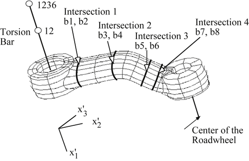
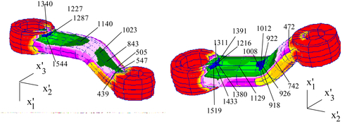
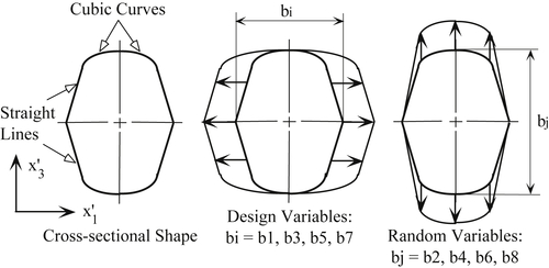
FIGURE 5.35 Roadarm finite element model.

FIGURE 5.36 Fringe plots of crack initiation life.

Table 5.5

Objective and Critical Constraint Functions

Function	Description	Lower Bound	Current Design	Status
Objective	Volume		487.678 in.³
Constraint 1	Node 1216	9.63 × 10⁶ (20 years)	9.631 × 10⁶ bks	Active
Constraint 2	Node 926	9.63 × 10⁶ (20 years)	8.309 × 10⁷ bks	Inactive
Constraint 3	Node 1544	9.63 × 10⁶ (20 years)	8.926 × 10⁷ bks	Inactive
Constraint 4	Node 1519	9.63 × 10⁶ (20 years)	1.447 × 10⁸ bks	Inactive
Constraint 5	Node 1433	9.63 × 10⁶ (20 years)	2.762 × 10⁸ bks	Inactive

For shape design parameterization, eight design variables are defined to characterize the geometric shapes of the four intersections, as shown in Figure 5.37. The profile of the crosssection shape is composed of four straight lines and four cubic curves. Side expansions

$(x_{1}^{'} - direction)$

of cross-sectional shapes are defined using design variables b1, b3, b5, and b7 for intersections 1 to 4, respectively. Vertical expansions

$(x_{3}^{'} - direction)$

of the cross-sectional shapes are defined using the remaining four design variables.

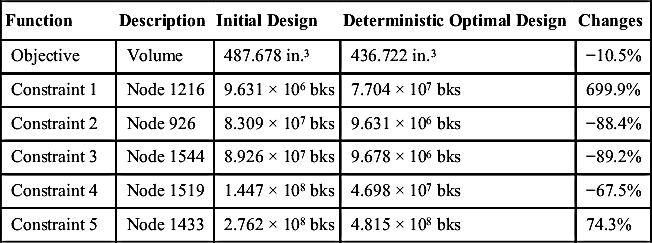
A deterministic optimal design is obtained in six design iterations using the modified feasible direction method in the design optimization tool (DOT). As shown in Table 5.6, at the deterministic optimal design, all fatigue lives are greater than the lower bound and objective function is reduced by 10.5%. The geometric shapes of the roadarm at initial and deterministic optimal designs are shown in Figure 5.38.

5.6.1.3.2. Probabilistic fatigue life predictions

The random variables and their statistical values for the crack initiation life predictions are listed in Table 5.7, including material and tolerance random variables. The eight tolerance random variables b1 to b8 are defined corresponding to the eight shape design variables defined in Figure 5.37.

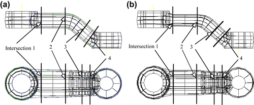
FIGURE 5.38 Geometric shape of the roadarm in front and top views. (a) Initial design. (b) Deterministic optimal design.

Table 5.6

Objective and Critical Constraint Function Values at Initial and Deterministic Optimal Designs

Function	Description	Initial Design	Deterministic Optimal Design	Changes
Objective	Volume	487.678 in.³	436.722 in.³	−10.5%
Constraint 1	Node 1216	9.631 × 10⁶ bks	7.704 × 10⁷ bks	699.9%
Constraint 2	Node 926	8.309 × 10⁷ bks	9.631 × 10⁶ bks	−88.4%
Constraint 3	Node 1544	8.926 × 10⁷ bks	9.678 × 10⁶ bks	−89.2%
Constraint 4	Node 1519	1.447 × 10⁸ bks	4.698 × 10⁷ bks	−67.5%
Constraint 5	Node 1433	2.762 × 10⁸ bks	4.815 × 10⁸ bks	74.3%

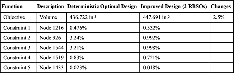
FORM is used to calculate the reliability of the crack initiation life at five critical points. The results shown in Table 5.8 indicate that the failure probability at nodes 926 and 1544 is greater than 3%. Because the failure probability of the roadarm at the deterministic optimal design is too high, a reliability-based design must be conducted to reduce the failure probability (to obtain a feasible design).

5.6.1.3.3. Reliability-based design

For the reliability-based design, the mean values of the eight shape parameters shown in Figure 5.37 are chosen as the design variables. The objective function is still the structural volume. The constraint functions are the failure probability of the fatigue life at the five critical points, with an upper bound of 1% (i.e., the required reliability of fatigue life larger than 20 years is 99%). Table 5.8 shows that the initial design is infeasible because the second and third constraints are violated. The reliability-based design sensitivity analysis (DSA) method discussed above is used to calculate the sensitivity coefficients of the fatigue failure probability with respect to the design variables.

Table 5.7

Definition of Random Variables

Random Variables	Mean Value	Standard Deviation	Distribution
Young's modulus E (psi)	30.0 × 10⁶	0.75 × 10⁶	LogNormal
Fatigue strength coefficient σ′_f	1.77 × 10⁵	0.885 × 10⁴	LogNormal
Fatigue ductility coefficient ε′_f	0.41	0.0205	LogNormal
Fatigue strength exponent b	−0.07300	0.00365	Normal
Fatigue ductility exponent c	−0.6	0.003	Normal
Tolerance b1 (in.)	2.889	0.032450	Normal
Tolerance b2 (in.)	1.583	0.019675	Normal
Tolerance b3 (in.)	2.911	0.031703	Normal
Tolerance b4 (in.)	1.637	0.019675	Normal
Tolerance b5 (in.)	2.870	0.031703	Normal
Tolerance b6 (in.)	2.420	0.026352	Normal
Tolerance b7 (in.)	2.801	0.032496	Normal
Tolerance b8 (in.)	4.700	0.050568	Normal

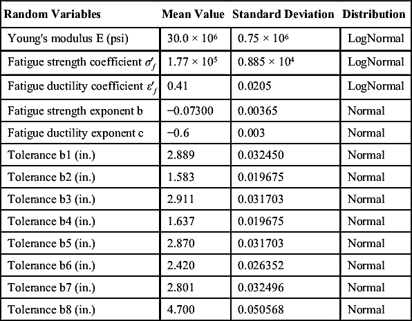
Table 5.8

Objective and Failure Function Values at Deterministic Optimal and Improved Designs

Function	Description	Deterministic Optimal Design	Improved Design (2 RBSOs)	Changes
Objective	Volume	436.722 in.³	447.691 in.³	2.5%
Constraint 1	Node 1216	0.476%	0.532%
Constraint 2	Node 926	3.24%	0.992%
Constraint 3	Node 1544	3.21%	0.998%
Constraint 4	Node 1519	0.83%	0.721%
Constraint 5	Node 1433	0.023%	0.018%

Because the current design is infeasible, a constraint correction algorithm is selected for the trade-off analysis. Using the sensitivity coefficients, a QP (quadratic programming) subproblem is employed to search a direction in which the reliability will quickly increase. Then, a what-if study is performed along the search direction suggested by the trade-off study, plus a step size.

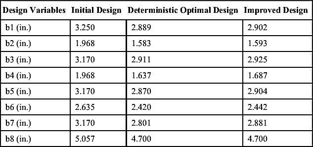
Through two iterations, a feasible design is achieved, as shown in Table 5.9. The two design iterations took 10 FORMs and two reliability-based DSAs. At the improved design, failure probabilities at five critical points are less than 1%, with 2.5% increments in volume. However, the total volume savings starting from the initial design is 8%—that is, from 487 in.³ to 447 in.³. The design variable values of the initial, deterministic optimal, and improved (after two interactive RBDOs) designs are listed in Table 5.9.

Table 5.9

Design Variable Values at Initial, Deterministic Optimal, and Improved Designs

Design Variables	Initial Design	Deterministic Optimal Design	Improved Design
b1 (in.)	3.250	2.889	2.902
b2 (in.)	1.968	1.583	1.593
b3 (in.)	3.170	2.911	2.925
b4 (in.)	1.968	1.637	1.687
b5 (in.)	3.170	2.870	2.904
b6 (in.)	2.635	2.420	2.442
b7 (in.)	3.170	2.801	2.881
b8 (in.)	5.057	4.700	4.700

5.6.2. Design Optimization for Structural Performance and Manufacturing Cost

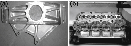
In mechanical and aerospace industries, engineers often confront the challenge of designing components that can sustain structural loads and meet the functional requirements (e.g., automotive suspension and engine components). It is imperative that these components contain the minimum material to reduce cost and increase efficiency of the mechanical system, such as fuel consumption. The geometry of these components is usually complicated due to strength and efficiency requirements, which often results in increased manufacturing time and cost. Some of these structural components are shown in Figure 5.39.

Although structural optimization has been widely used for many decades to solve such problems, the primary focus has been on the functionality aspects of the design. During the course of an optimization, the geometric complexity of the component may increase, making manufacturing difficult or uneconomical. Due to the increasing geometric complexity, conventional structural optimization problems that define mass as the objective function may not yield components with minimum cost from the manufacturing perspective. This especially holds true for machined components because machining cost is often the dominant constituent of product cost for such components.

FIGURE 5.39 Mechanical components involving time-consuming and precision machining operations. (a) Upright in an automotive suspension. (b) Engine block.

In this subsection, we present a case study of structural shape optimization that incorporates machining and material costs as the objective function subject to structural performance constraints. Structural shape optimization reduces material, but it may be accompanied by increases in the geometric complexity due to changes in the design boundary, which ultimately increases manufacturing cost. In this case study, we present a design process that incorporates manufacturing costs into structural shape optimization and produces components that are cost effective and satisfy specified structural performance requirements.

5.6.2.1. Design problem definition and optimization process

As discussed in Chapter 3, a typical single-objective optimization problem is defined as follows:

$Minimize : f (b)$

(5.57a)

$Subject to : g_{i} (b) \leq 0, i = 1, m$

(5.57b)

$h_{j} (b) = 0, j = 1, p$

(5.57c)

$b_{k}^{ℓ} \leq b_{k} \leq b_{k}^{u}, k = 1, n$

(5.57d)

where f(b) is the objective function; b is the vector of design variables, g_i(b) is the ith inequality constraint, and h_j(b) is the jth equality constraint. The objective function f(b) is the product cost for the component to be discussed shortly.

It is assumed that the designer has all of the required data, such as the initial shape of the component, boundary and loading conditions, material properties, and machining sequences. A solid model of the component is created using solid features in CAD software. Dimensions of the solid features also serve as design variables for the optimization problem. A virtual machining (VM) model is created by defining appropriate machining operations and sequences based on the given solid model. The machining parameters specific to each machining sequence are also specified in the VM model. Similarly, an FEA model is constructed using given boundary and loading conditions, as well as initial geometric information.

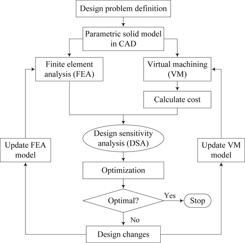
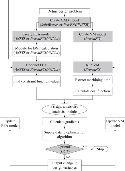
The design velocity field is then computed for sensitivity analysis and finite element mesh updates. FEA and VM are conducted to evaluate structural and machining performance measures, respectively. Machining time obtained from the VM model is important for the calculation of machining costs. Data obtained from FEA and VM models are used to evaluate objective and constraint functions. Design sensitivity analysis is conducted to compute the gradients of the objective function and constraints with respect to changes in the design variables. The gradients and values of the objective and constraint functions are passed to an optimization algorithm, which determines the design changes for the next design iteration. FEA and VM models are then updated using these changes, and the process is iterated as shown in Figure 5.40, until an optimal design is achieved.

FIGURE 5.40 The design optimization process.

5.6.2.2. Manufacturing cost model

The objective function f(b) in Eq. 5.57a is defined as follows (Edke and Chang 2006):

$f (b) = C_{mat} γ V (b) + C_{mc} τ (b) + C_{t}$

(5.58)

where the three terms on the right-hand side represent material cost, machining cost, and tooling cost, respectively. In Eq. 5.58, C_mat is the material cost rate ($/lb); γ is the specific weight of the material; V(b) is the volume of the component that depends on design; C_mc is the machining cost rate ($/min); τ(b) is the time required to machine one component, which also depends on design; and C_t is the tooling cost ($).

The machining cost rate accounts for the cost of actual machining operations, machine shop overheads, operator wages and overheads, indirect costs such as cost of electricity, and machine depreciation (Dieter 1991). C_mc is given as

$C_{mc} = \frac{1}{60} [\frac{M (100 + O H_{M})}{100} + \frac{W (100 + O H_{OP})}{100}]$

(5.59)

In this equation, M is the cost of machine operation per hour ($/h); OH_M is the machine overhead rate (%); W is the hourly wage for the operator ($/h); and OH_OP is operator overhead rate (%). The unit time τ(b) in Eq. 5.58 is the sum of machining time t_mc and idle time t_i: τ = t_mc + t_i, in which

$t_{mc} = (\frac{L}{v_{f}} + \frac{L^{'}}{v_{r}}); and t_{i} = t_{set} + t_{ch} + t_{hand} + t_{down} + t_{ins}$

(5.60)

In Eq. 5.60, L is the total tool travel while cutting (m); L′ is the tool travel during rapid traverse (m); v_f is the feed rate (m/min); v_r is the rapid traverse velocity (m/min); t_set is the job setup time per part (min); t_ch is the time for tool change (min); t_hand is the work-piece handling time (min); t_down is the machine down time (min); and t_ins is the time for in-process inspection (min). The cost of tooling, which includes cost of cutting tools and cost of jigs/fixtures, is given as

$C_{t} = \frac{t_{mc}}{T_{tl}} (\frac{K_{i}}{n_{i}} + \frac{K_{h}}{n_{h}}) + C_{f}$

(5.61)

where T_tl is the total tool life (min); K_i is cost of the insert ($); n_i is the number of cutting edges; K_h is the tool holder cost ($); n_h is the number of cutting edges in the tool-holder; and C_f is the cost of jigs/fixtures ($). Machining time t_mc is obtained from VM. Similarly, cost models for other machining processes can be developed.

5.6.2.3. Virtual manufacturing

Virtual manufacturing is a simulation-based method that supports engineers to define, simulate, and visualize the manufacturing process in a computer environment. By using virtual manufacturing, the manufacturing process can be defined and verified early in the design process. In addition, the manufacturing time can be estimated. Material cost and manufacturing time constitute a significant portion of the product cost. The virtual machining operations, such as milling, turning, and drilling, allow designers to conduct machining process planning, generate machining tool paths, visualize and simulate machining operations, and estimate machining time. Moreover, the tool path generated can be converted into Computer Numerical Control (CNC) codes (M-codes and G-codes) (Lee 1999; Chang 2013b) and loaded to CNC machines, such as HAAS mills (www.haascnc.com), to machine functional parts as well as dies or molds for production.

Geometrically complex parts are commonly found in the automotive and aerospace industries, where molds and dies are manufactured. The time taken to manufacture molds or dies of different sizes and complexities ranges from 1200 to 3800 h (Sarma and Dutta 1997). Considerable time (49–72%) is spent in contour surface milling for the design surfaces (the surfaces to be machined) of molds and dies (Sarma and Dutta 1997). Design changes in structural geometry due to functional considerations may affect the manufacturing cost significantly. Among different types of machining processes, contour surface milling is most applicable for mold and die machining. Existing commercial CAM tools, such as Pro/MFG (www.ptc.com), support contour surface milling using various methods, including isoparametric (Kai et al. 1995), constant curvature (Lo and Hsaio 1998), and constant scallop height (Sarma and Dutta 1997).

Typical milling operations that make molds or dies include pocket milling and surface contour milling. The quality and accuracy of the machined surfaces are largely determined by surface contour milling. In this section, surface contour milling will be briefly discussed to illustrate the connection between manufacturing time and structural geometric shape determined by performance requirements.

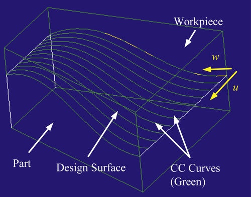
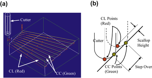
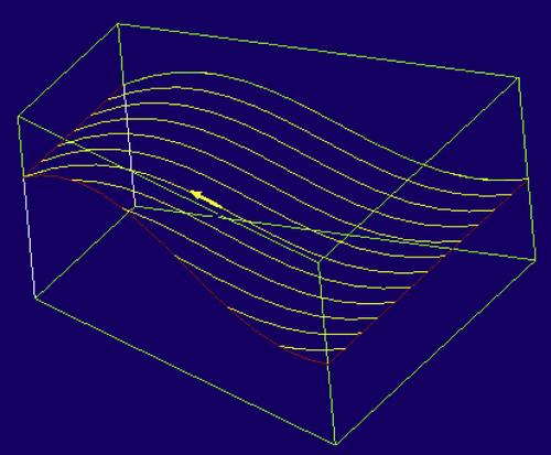
As discussed in Chapter 4, parametric surfaces are employed to parameterize the design boundary. The same surfaces will be assumed for machining. In general, the cutter contact (CC) curves are first generated on the design surface, as shown in Figure 5.41. The CC curves are created, for example, by uniformly splitting parameter u or w:

$C^{i} (w) = S (u_{i}, w), u_{i} \in [u_{min}, u_{max}]$

(5.62)

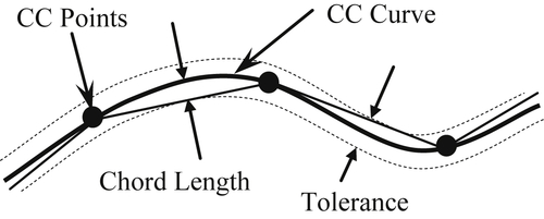
where Cⁱ(w) is the ith CC curve (which is indeed a u-isoline), and S(u, w) is the parametric design surface. The CC points are discrete points generated along the CC curve, which form a piecewise linear approximation of the CC curve for the CNC controller to trace. The chord length between the CC curve and the polyline formed by the CC points must be less than a prescribed tolerance, as illustrated in Figure 5.42. CL (cutter location) points are then obtained by offsetting from the CC points, considering workcell and cutter shape, as illustrated in Figure 5.43.

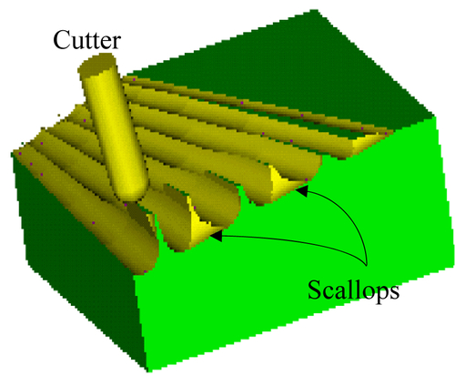
FIGURE 5.41 Design surface and CC curves.

Machining time t_mc can be estimated by the length of the CL polyline and a prescribed feed rate. As can be seen in Figure 5.44, scallops remaining on the design surface are not uniform. A uniform scallop (with constant scallop height) is more desirable for the follow-on grinding operations. This can be reasonably achieved by moving the cutter on the design surface with a uniform physical spacing, as illustrated in Figure 5.45.

5.6.2.4. Design sensitivity analysis

As discussed in Chapter 4, design sensitivity analysis calculates the gradients of the objective and constraint functions with respect to design variables. Shape sensitivity analysis for structural performance measures has been developed for many years (Choi and Kim 2006) and was briefly discussed in Chapter 4. Sensitivity of machining time due to changes in the design surface can be calculated for specific machining sequences. For example, sensitivity analysis of machining time for a contour surface milling using the isoparametric method can be obtained as follows. First, a new parametric surface will be generated for a small design change of the kth design variable δb_k. The CC curves on the perturbed parametric surface can be created by

FIGURE 5.43 Offset CC for CL points: (a) CL and CC lines (3-axis mill) and (b) cutter offset and scallop.

$C^{i} (w; b + δ b_{k}) = S (u^{i}, w; b + δ b_{k}), u^{i} \in [u_{min}, u_{max}]$

(5.63)

where uⁱ is the u-parametric coordinate of the ith CC curve, which is kept the same before and after the design perturbation. Following the procedures discussed above, CC points and CL points are calculated next, considering chord length tolerance, workcell, and cutter shape. The new machining time t_mc(b + δb_k) can then be calculated by multiplying the length of the polyline formed by the new CL points with the same prescribed feed rate. The sensitivity of the machining time can be approximated by

$\frac{\partial t_{mc}}{\partial b_{k}} \approx \frac{t_{mc} (b + δ b_{k}) - t_{mc} (b)}{δ b_{k}}$

(5.64)

However, the overall finite difference method is probably more general and more straightforward to implement in CAM, especially while considering other machining sequences, such as constant scallop height surface contour milling.

5.6.2.5. Software implementation

The design optimization process is implemented using commercial CAD/CAM/FEA and design optimization tools, as illustrated in Figure 5.46. The shaded boxes show the commercial tools, while the plain boxes show software modules that need to be developed.

As a sample implementation (Edke and Chang 2006), SolidWorks and Pro/ENGINEER were selected for CAD modeling, ANSYS (www.ansys.com) and Pro/MECHANICA (www.ptc.com) for finite element modeling, Pro/MFG for virtual machining, and DOT for optimization. MATLAB and C/C++ are used to construct application programs for data transfer and mathematical computations.

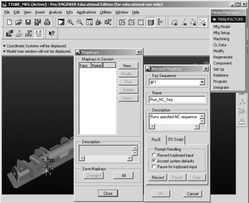
Note that after a change is made in model dimensions, Pro/MFG updates the tool path for an NC sequence only after the particular NC (numerical control) sequence is run. This is when the tool path computations for that NC sequence are performed. Although most of the automation in Pro/ENGINEER can be achieved using Pro/TOOLKIT (e.g., for CAD model updates), Pro/TOOLKIT does not provide any function to perform the tool path computations. Tool path generation in Pro/MFG has to be done interactively by making a series Pro/ENGINEER menu and dialogue box selections. To overcome this problem, the “mapkeys” feature in Pro/ENGINEER is used.

Mapkeys are similar to the macros used in many application packages. A mapkey is a keyboard macro that maps frequently used command sequences to certain sets of keyboard keys. The approach for the recording of a mapkey and its value is shown in Figure 5.47 as an example. Once a mapkey is recorded, it is saved in a configuration file mapkey, with each macro beginning on a new line. Value of this mapkey (the string of commands) can be copied into a Pro/TOOLKIT application as a command string. Using a Pro/TOOLKIT function, the commands are loaded into a stack and are executed sequentially after the control returns to Pro/ENGINEER from the Pro/TOOLKIT application. Using these mapkeys, a Pro/TOOLKIT application is constructed to run the machining sequences and to extract total machining time.

FIGURE 5.46 Optimization flow with required software modules.

5.6.2.6. Aircraft torque tube example

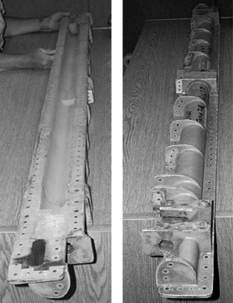
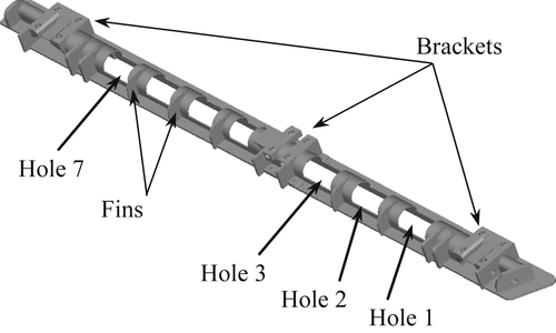
The torque tube shown in Figure 5.48 is a structural component located inside the wings of an aircraft. Loads are applied to the three brackets and the bottom face of the tube is bolted to the wing flap. The tube is made up of AL2024-T351 with yield strength of 43 ksi. Seven rectangular holes are created between fins to reduce the weight of the torque tube, as shown in Figure 5.49.

FIGURE 5.47 Recording a mapkey in Pro/ENGINEER.

5.6.2.6.1. Problem definition

The objective of the torque tube optimization problem is to minimize the product cost subject to limits on structural performance measures. The objective function, which is similar to Eq. 5.58, is defined as:

$\begin{matrix} Minimize : & f (b) = C_{mat} γ {V_{0} - [5 V_{1} (b_{1,}, b_{2}) - V_{2} (b_{3}, b_{4}) - V_{3} (b_{5,}, b_{6})]} \\ + \frac{1}{60} (t_{mc} + t_{i}) [\frac{M (100 + O H_{M})}{100} + \frac{M (100 + O H_{OP})}{100}] \end{matrix}$

(5.65a)

$Subject to : σ_{1 max} (b), σ_{2 max} (b), \dots, σ_{12 max} (b) \leq 21.5 ksi$

(5.65b)

$b_{j}^{ℓ} \leq b_{j} \leq b_{j}^{u}, j = 1,6$

(5.65c)

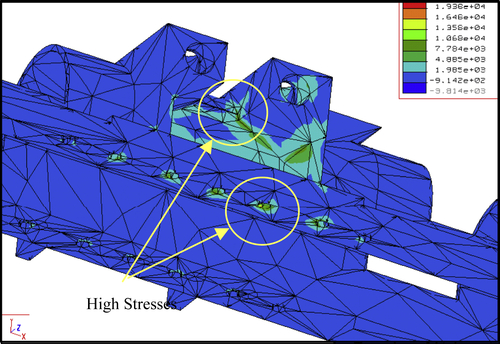
Note that tooling cost is ignored in this problem for simplicity. The tube volume is computed by subtracting the volume of holes from its total volume. Since the five holes (1, 2, 5, 6, and 7) are grouped together, they have only two design variables in common. The maximum principal stresses at 12 locations are defined as constraint functions (see Figure 5.51 for some of the high stresses). The limit on the maximum stress is 21.5 ksi. It is apparent that changes in the hole sizes will vary the weight of the tube, may impact the structural integrity, and influence machining time of the tube. The design variable bounds are listed in Table 5.10.

5.6.2.6.2. Design parameterization

Parameterization of the torque tube holes is shown in Figure 5.50. Hole depth and half of the hole length are selected as design variables. When the length of the holes is changed, the holes either expand or contract symmetrically. Also, the position of the hole is maintained such that it always remains centered between the adjacent fins. From initial tests, it was observed that the maximum stress occurs near the middle bracket. Hence, except for the two holes adjacent to the middle bracket, the design variables of all other holes are grouped together; implying that width and length of the Holes 1, 2, 5, 6, and 7 are changed at the same amounts, respectively. This reduces the number of design variables from 14 (2 design variables per hole time 7 holes) to 6.

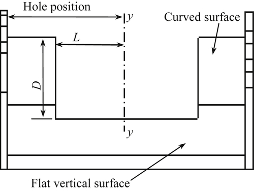
FIGURE 5.50 Parameterization of torque tube holes.

Table 5.10

Upper and Lower Bounds of Design Variables for the Torque Tube

	Lower Limit (in.)	Upper Limit (in.)
b1 (length of holes 1, 2, 5, 6, and 7)	0.90	2.30
b2 (depth of holes 1, 2, 5, 6, and 7)	1.50	1.95
b3 (length of hole 3)	1.10	2.50
b4 (depth of hole 3)	1.50	1.95
b5 (length of hole 4)	0.60	1.40
b6 (depth of hole 4)	1.50	1.95

5.6.2.6.3. Finite element analysis

The finite element model constructed in Pro/MECHANICA consists of 11,502 elements. A p-convergence study is conducted at the outset to fix the polynomial level of the element shape function for the analysis. The criterion specified is 3.5% strain energy convergence. The polynomial order is fixed at 7. The FEA solves 2,242,623 equations. Because the model is constrained by fixing displacements at finite element nodes at some locations, concentrated high stresses at such nodes are neglected.

The highest maximum principal stress is located at one of the holes and the inner edge of the middle bracket, as shown in Figure 5.51. The maximum stress magnitude is 20.70 ksi, which is close to the constraint limit (21.5 ksi). Note that a safety factor of 2 is used.

The most critical information required for performing design optimization in this example is the design velocity field. Once the velocity field is obtained, the remaining optimization process becomes routine. For the torque tube, the design boundaries (hole surfaces) are plane surfaces, as shown in Figure 5.52. This simplifies the velocity field calculations, as the prescribed displacement itself is now the boundary velocity. Thus, only domain velocity field calculation is required.

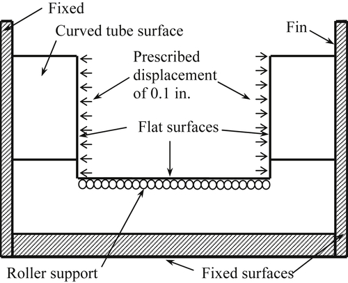
FIGURE 5.51 Finite element analysis results.

FIGURE 5.52 Velocity field computation for length design variables.

As shown in Figure 5.52, the fins and bottom surfaces are fixed. For the length design variables, a prescribed displacement of 0.1 in. is applied on the two end surfaces of the hole along the longitudinal direction. Roller boundary conditions are applied to the bottom surface of the holes. FEA is conducted to calculate the displacement of the finite element nodes, which is the design velocity field of the length design variable. To calculate the design velocity of the depth design variable, a prescribed displacement of 0.1 in. is applied to the bottom surface of the holes, and the two longitudinal end surfaces are fixed.

Table 5.11

Machining Parameters and Machining Time

Parameter name	Value
Tool	0.5 in. end mill
Feed rate	10 in./min
Spindle speed	1250 rpm
Step depth	0.2 in.
Machining time (initial design)	41.26 min

5.6.2.6.4. Virtual machining

The VM model defined in Pro/MFG consists of an assembly of the torque tube without holes and the torque tube with holes. The machining parameters are summarized in Table 5.11. A customized pocket milling sequence (Figure 5.53) is defined in Pro/MFG to simulate the machining process. The time required to machine all the holes is 41.26 min for the initial values of design variables.

5.6.2.6.5. Design optimization

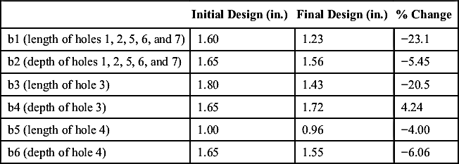
The sequential quadratic programming (SQP) algorithm is used for conducting design optimization. The convergence criterion is 1% of the objective function. The algorithm converges in four iterations. There is a 2.4% decrease in the cost. The weight of the torque tube reduces by 6.1%. Machining time decreases by 10.6%. The optimization history is shown in Figure 5.54. The values of the design variables for initial and final design are summarized in Table 5.12.

The design process presented successfully incorporates machining cost into a structural shape optimization problem. In addition to ensuring the manufacturability of the optimized components, the design process delivers components with a minimum cost and the required performance. The trade-off between structural performance and machining cost is critical, as revealed in this torque tube example.

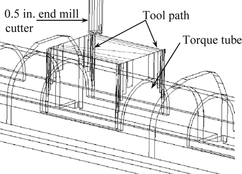
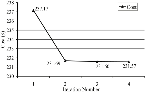
FIGURE 5.53 Virtual machining in Pro/MFG.

Table 5.12

Optimization Results for the Torque Tube

	Initial Design (in.)	Final Design (in.)	% Change
b1 (length of holes 1, 2, 5, 6, and 7)	1.60	1.23	−23.1
b2 (depth of holes 1, 2, 5, 6, and 7)	1.65	1.56	−5.45
b3 (length of hole 3)	1.80	1.43	−20.5
b4 (depth of hole 3)	1.65	1.72	4.24
b5 (length of hole 4)	1.00	0.96	−4.00
b6 (depth of hole 4)	1.65	1.55	−6.06

..................Content has been hidden....................

You can't read the all page of ebook, please click here login for view all page.

Table of Contents for 5.6. Advanced Topics

Create new playlist

Sign In

Sign Up

5.6. Advanced Topics

5.6.1. Reliability-Based Design Optimization

5.6.1.1. Failure probability

5.6.1.2. RBDO problem formulation

5.6.1.2.1. Reliability-based design sensitivity analysis

5.6.1.3. RBDO for a tracked-vehicle roadarm

5.6.1.3.1. Deterministic design optimization

5.6.1.3.2. Probabilistic fatigue life predictions

5.6.1.3.3. Reliability-based design

5.6.2. Design Optimization for Structural Performance and Manufacturing Cost

5.6.2.1. Design problem definition and optimization process

5.6.2.2. Manufacturing cost model

5.6.2.3. Virtual manufacturing

5.6.2.4. Design sensitivity analysis

5.6.2.5. Software implementation

5.6.2.6. Aircraft torque tube example

5.6.2.6.1. Problem definition

5.6.2.6.2. Design parameterization

5.6.2.6.3. Finite element analysis

5.6.2.6.4. Virtual machining

5.6.2.6.5. Design optimization

Table of Contents for
5.6. Advanced Topics