
Project S5
Design with SolidWorks
Abstract
In Project S5, we introduce SolidWorks design optimization capabilities as well as conducting interactive design using the suite of SolidWorks CAD/CAE/CAM capabilities for a multidisciplinary design problem. We include an optimization design study for a cantilever beam as a single-objective optimization. Then we present a single-piston engine example to illustrate the interactive design process discussed in Chapter 3 involving multiple engineering disciplines. For those who are not familiar with SolidWorks and embedded CAE/CAM modules, we encourage you to go over Projects S1 to S4 of the book series before moving forward with this tutorial project. Without going over these prior projects, you may get lost very quickly. Example models are available for download at the book’s companion website.
Keywords
Multidisciplinary optimization; design optimization; sensitivity analysis; what-if studyDesign optimization was discussed in Chapters 3 and 5 for single-objective and multiobjective problems, respectively. In these chapters, both theoretical and practical aspects of the topics were discussed. With a basic understanding of the concept, theories, and solution techniques of design optimization, we are ready to go over a few tutorial lessons on design optimization capabilities offered by commercial tools, such as SolidWorks.
In Project S5, we introduce SolidWorks design optimization capabilities and then conduct interactive design using the suite of SolidWorks computer-aided design (CAD), engineering (CAE), and manufacturing (CAM) capabilities for a multidisciplinary design problem. We include an optimization design study for a cantilever beam as a single-objective optimization. Then, we present a single-piston engine example to illustrate the interactive design process discussed in Chapter 3 involving multiple engineering disciplines. For those who are not familiar with SolidWorks and embedded CAE/CAM modules, we encourage you to go over Projects S1–S4 of the book series before moving forward with this tutorial project. Without going over these prior projects, you may get lost very quickly. Example models are available for download at the book's companion Web site.
Overall, the objective of this project is to enable readers to use SolidWorks for batch-mode design optimization and interactive design. The use of the capability for design optimization should be straightforward. Those who are interested in learning more about the batch-mode optimization may go over a few more examples offered as YouTube videos, such as those listed below, subject to their availability.
▪ Design study and optimization in SolidWorks finite element analysis (FEA) by Intercad (http://www.youtube.com/watch?v=TJDvfvu0WRE)
▪ Torsional static analysis and design study example using SolidWorks (http://www.youtube.com/watch?v=KTWEDiwZwvs)
Note that the lessons included in this project were developed using SolidWorks 2013 SP2.0 and CAMWorks 2014. If you are using a different version of SolidWorks or CAMWorks, you may see slightly different menu options or dialog boxes.
S5.1. Introduction to Design Optimization in SolidWorks
There are two main modes for running a design study in SolidWorks: evaluation and optimization. Evaluation supports users in specifying discrete values for each variable and using sensors as constraints. The software runs the study using various combinations of the values and reports the output for each combination.
For example, consider the plate with a hole shown in Figure S5.1 for a design change. Using the evaluation capability, users may specify values of 0.2, 0.1, and 0.3 m for the length variable (currently L = 0.2 m); 0.1, 0.05, and 0.15 m for the height variable (currently H = 0.1 m); and 0.04, 0.02, and 0.06 m for the diameter variable (ϕ = 0.04 m). You can specify a volume sensor to monitor the volume of the plate. The design study results report the volume of the plate for each combination of L, H, and ϕ—in this case, 3 × 3 × 3 = 27 combinations.
Optimization, on the other hand, allows users to specify values for each variable, either as discrete values or as a range. Users use sensors as constraints and as goals. The software runs iterations of the values and reports the optimum combination of values to meet specified goal. Note that a sensor in SolidWorks monitors selected properties of parts and assemblies and alerts users when values deviate from the limits that users specify. Sensors can be used to study mass properties, dimensions, interface detection, proximity (available in assemblies only for monitoring the assembly for interferences between components users select), simulation data, and motion data.
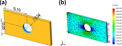
For example, for the plate model described earlier, users specify a range of 0.1–0.3 m for the length variable (L); discrete values of 0.1, 0.05, and 0.15 m for the height variable (H); and a range of 0.04–0.06 m for the diameter variable (ϕ = 0.04 m). For a constraint, one specifies a stress sensor to be less than 380 MPa, and uses a mass sensor to minimize the mass of the plate. The optimization design study iterates on the values specified for L, H, ϕ, and stress, then reports the optimum combination to produce the minimum mass that satisfies the stress constraint. In this tutorial project, we focus only on the optimization of the design study.
We use a cantilever beam example for illustration of the optimization capability (batch mode) in Section S5.2. The beam example is a single-objective optimization problem of a single discipline, only involving structural performance measures. In addition, we use a single-piston engine example in Section S5.3 to illustrate the details of a multidisciplinary design problem using an interactive design process, in which structural, motion, and manufacturing are involved.
The main objective of this tutorial project is to help you, as an experienced SolidWorks user, become familiar with SolidWorks design optimization capabilities. The discussion on SolidWorks software, including motion, simulation, and CAMWorks, in this section will be brief.
S5.1.1. Defining an Optimization Problem
As discussed in Chapter 3, a single-objective optimization problem can be formulated mathematically as follows:
![]() (S5.1a)
(S5.1a)
![]() (S5.1b)
(S5.1b)
![]() (S5.1c)
(S5.1c)
![]() (S5.1d)
(S5.1d)
where f(x) is the objective function or goal to be minimized (or maximized); gi(x) is the ith inequality constraint; m is the total number of inequality constraint functions; hj(x) is the jth equality constraint; p is the total number of equality constraints; x is the vector of design variables, with x = [x1, x2, ..., xn]T; n is the total number of design variables; and  and
and  are the lower and upper bounds of the kth design variable xk, respectively.
SolidWorks supports users in defining an optimization problem, running the optimization (using the so-called generative method, as discussed in Chapter 3), and displaying optimization results. Note that if you plan to use simulation data sensors, you must create at least one initial simulation study before creating the design study.
A design study can be initiated by choosing from the pull-down menu:
Insert > Design Study > Add.
In the Design Study Manager window shown in Figure S5.2, users define an optimization problem by entering and choosing objective (goals), constraints, and variables using the Variable View tab or Table View tab. Results view allows users to view optimization results in tables or graphs.
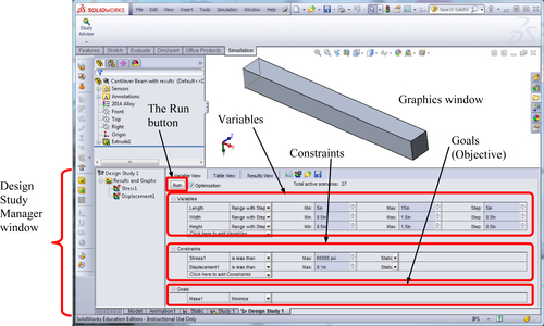

Goals can be chosen from a predefined sensor. Users may add more sensors to goals. For multiple goals, users may enter the weight of each goal. For example, in Figure S5.3, mass and displacement are included in the goals with weights of 3 and 1, respectively. The weight of a goal represents its relative importance. The higher the weight of the goal, the more important it is to optimize that goal. The program normalizes the weights and uses the weight-sum method discussed in Chapter 5 to conduct multiobjective optimization.
Users may choose continuous variables to perform optimization. For each design variable, users need to define its lower and upper limits, as well as step size to vary. Dimensions of the solid model are the most common variables for optimization. In addition, parameters, such as material properties, can be chosen as design variables. Note that the model, part, or assembly must be fully parameterized to conduct a batch-mode optimization in SolidWorks, as discussed in Chapter 3. For more about design parameterization, the reader is referred to Chang (2014a).
Similar to goals, you may choose sensors to define constraints. For the condition, you may select one of the following four constraints: (1) “monitor only,” monitoring the sensor value without imposing any constraints; (2) “is greater than” the minimum acceptable sensor value; (3) “is less than” the maximum acceptable sensor value; and (4) “is between” the range of acceptable sensor values.
Once an optimization problem is completely defined, users may simply click the Run button above the Variable table (see Figure S5.1) to launch an optimization run.
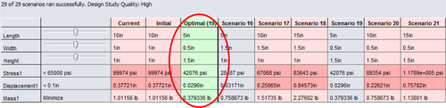
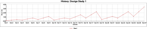
At the end of the run, users may choose the Results View tab to review the results of the study, such as those shown in Figure S5.4. Users may click a scenario to update the model in the graphics window with the variables of that scenario. A green-colored scenario indicates the best or optimal result. A red color indicates a violation of one or more constraints by the scenario. A background color indicates the current scenario and all scenarios that are not optimal. Users may also create graphs to see optimization history, like the one shown in Figure S5.5. Note that although the graph is called “history,” it is nothing but a polyline that connects results of individual scenarios.
S5.1.2. Tutorial Examples
Two examples are included in this tutorial project. The first example, a cantilever beam, illustrates step-by-step details of defining an optimization problem, running optimization, and showing results in table and graphs. The second example, a single-piston engine, illustrates an interactive design process of solving a multidisciplinary design problem using SolidWorks Simulation, motion, CAMWorks, the sensitivity display, and a what-if study, discussed in Chapter 3. Because the detailed steps in using individual software modules have been discussed in Projects S1–S4, we only include major steps with key information in these examples. Examples and topics to be discussed in each lesson are summarized in Table S5.1.
Table S5.1
Examples Employed in This Project
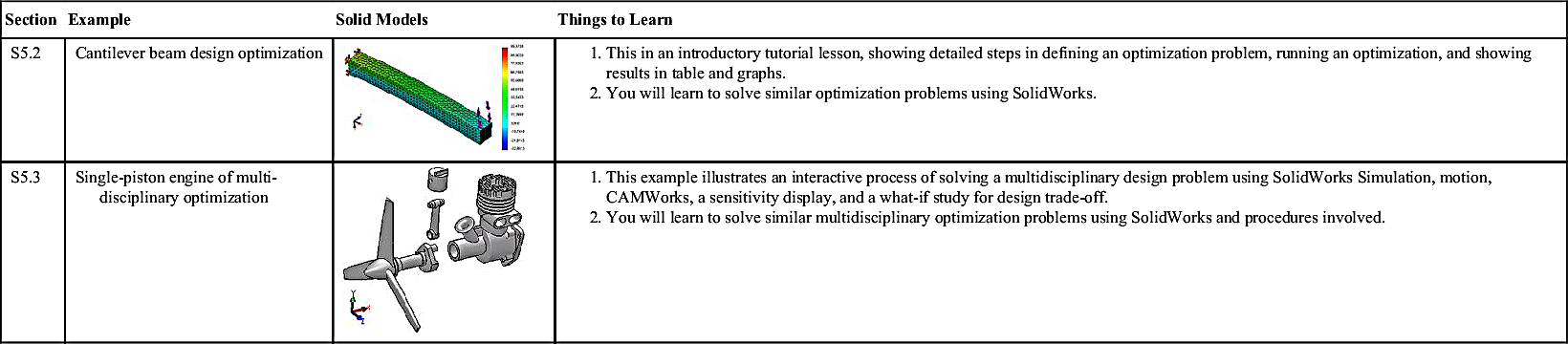
S5.2. Cantilever Beam
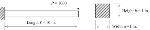
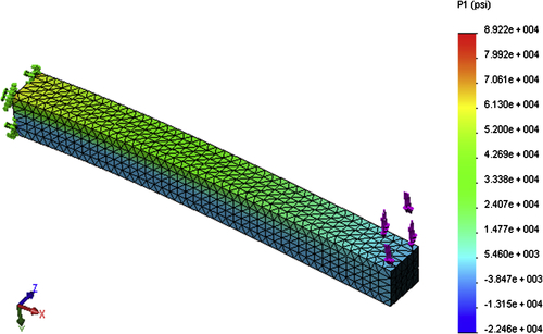
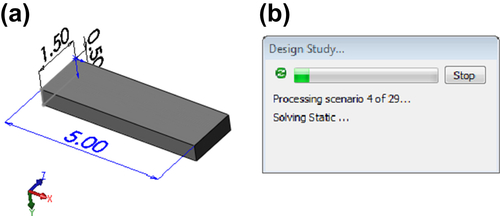
We use the cantilever beam example from Chapter 3 to illustrate the steps for carrying out design optimization using SolidWorks. The beam is shown again in Figure S5.6. The beam is made of cast stainless steel. In the current design, the beam length  and the width w and height h of the crosssectional area are both 1 in. The load is P = 1000 lbf acting at the tip of the beam, as shown in Figure S5.6. Our goal is to optimize the beam design for a minimum mass subject to displacement and stress constraints by varying its length as well as the width and height of the crosssection.
S5.2.1. Design Problem Definition
The design problem of the cantilever beam example is formulated mathematically as:
![]() (S5.2a)
(S5.2a)
![]() (S5.2b)
(S5.2b)
![]() (S5.2c)
(S5.2c)
![]() (S5.2d)
(S5.2d)
in which ρ is the mass density, σmp is the maximum principal stress, and δy is the maximum displacement in the Y-direction (vertical).
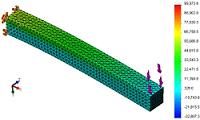
A static design study is created for the beam, with the boundary and load conditions shown in Figure S5.7. The material chosen is cast stainless steel from the simulation material library. The unit system chosen is IPS (in.-lbf-s). Also shown in Figure S5.7 are the finite element mesh (default median mesh) and the fringe plot of the maximum principal stress (or first principal stress).
In the current design, the maximum principal stress (g1) is 89.2 ksi, which is greater than the required upper bound of 65 ksi (tensile strength, assumed). This performance constraint is violated (hence, design is infeasible).
The second performance constraint of maximum y-displacement (g2) is 0.1454 in., which is greater than the required upper bound of 0.1 in. Again, this performance constraint is violated (design is infeasible).
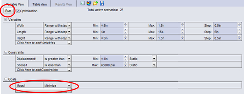
We are changing the width, height, and length of the beam to find an optimal solution. We choose a 0.5-in. step size for varying the width and height design variables, and a 5-in. step size for the length design variable. As a result, each design variable is varied three times. For example, the width design variable is changed from its lower bound of 0.5 in. to 1 in., and then to its upper bound of 1.5 in. Similarly, three changes take place for the height and length design variables, respectively. These changes in design variables are combined to create 27 (3 × 3 × 3) scenarios to search for a possible optimal solution.
A total of 29 static analyses (27 plus the initial and current designs) will be carried out for the study. In the graphics window, the design of all scenarios will appear in the beam with changing dimensions.
S5.2.2. Using SolidWorks
S5.2.2.1. Open SolidWorks part
Open the solid model of the cantilever beam downloaded from the book companion Web site, filename: Cantilever Beam.SLDPRT in folder: Project S5 Examples/Lesson S5.2 Cantilever Beam. This cantilever example is similar to that of Project S3.2 of Chang (2013a). After opening this file, you should see that there is already a static study created for you. You may want to browse the stress and displacement results of the study. Also, please check the unit system (IPS), and take a look at the finite element mesh.
S5.2.2.2. Insert a design study
From the pull-down menu, choose
Insert > Design Study > Add
and name the study My_Opt.
S5.2.2.3. Add design variables
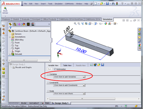
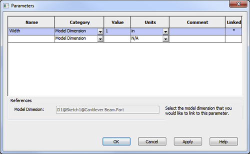
In the Design Study Manager window (Figure S5.8), click “Click here to add variables” under Variables, and choose Add Parameter to add design variable. In the Parameters dialog box (Figure S5.9), enter Width for name, and then pick the width dimension from the solid model in the graphics window. The selected dimension should appear under Value in the Parameters dialog box (Figure S5.9). Click Apply to accept the parameter.
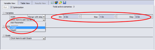
In the Design Study Manager window (Figure S5.10), Min, Max, and Step (0.5, 1.5, and 0.5 in., respectively) are automatically added to the length design variable. These are lower and upper bounds of the width design variable. Step: 0.5 in. implies that the design will be changed for every 0.5 in. We will stay with this default setup.
Repeat the same steps to define the height and length dimensions. All three variables should appear in the Parameters dialog box. Click OK to close the Parameters dialog box.
You may select Height and Length parameters in the Design Study Manager window, and review their respective Min, Max, and Step values.
S5.2.2.4. Add constraints
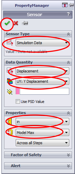
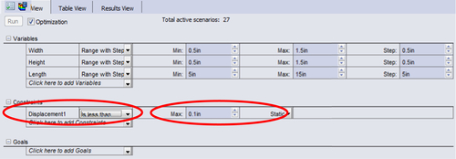
In the Design Study Manager window (Figure S5.8), click “Click here to add constraints” under Constraints, and choose Add Sensor to add a constraint. In the Property Manager dialog box (Figure S5.11), choose Simulation Data, Displacement, UY: Y Displacement, in, Model Max, and then Accept (checkmark). The constraint should appear in the Design Study Manager window, under Constraints. Choose “Is less than,” and enter 0.1 in. for its upper bound (see Figure S5.12).
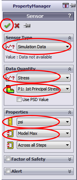
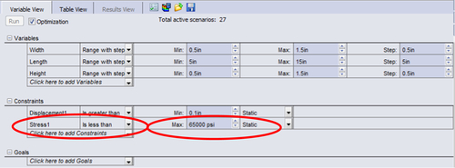
Repeat the same to create a stress constraint by choosing Simulation Data, Stress, P1: 1st Principal Stress, psi, Model Max (see Figure S5.13). The stress constraint should appear in the Design Study Manager window, under Constraints. Choose “Is less than,” and enter 65,000 psi for its upper bound (Figure S5.14).
S5.2.2.5. Add objective functions (Goal)
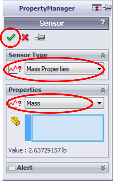
In the Design Study Manager window, click “Click here to add goals” under Goals, and choose Add Sensor. In the Property Manager dialog box (Figure S5.15), choose Mass Properties, Mass, and then Accept (checkmark). The goal should appear in the Design Study Manager window, under Goals (Figure S5.16) with Minimize condition. At this point, we have completed the definition of the design problem. We are ready to carry out an optimization for this beam example.
S5.2.2.6. Run optimization
In the Design Study Manager window, click Run (Figure S5.16). Design variables will be varied one at a time in accordance with the limits and steps as defined earlier. A total of 29 static analyses (27 plus initial and current) will be carried out for the study. In the graphics window, design of all scenarios will appear sequentially (e.g., see Figure S5.17).
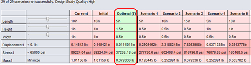
At the end, an optimal design is found for Scenario 7 (see Figure S5.18), in which width, height, and length become 0.5, 1.5, and 5 in., respectively. Displacement is 0.0114 in. (<0.1 in.), stress is 37,238 psi (<65 ksi), and the total mass is 0.379 lbm (reduced from 1.012 lbm from the initial design).
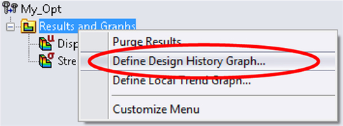
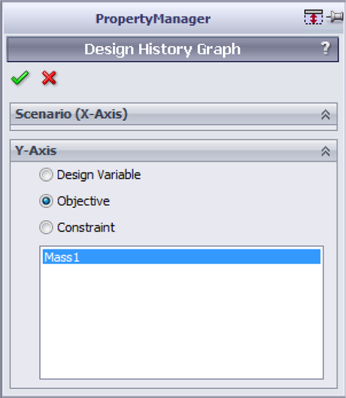
In the Design Study Manager window, right-click the Results and Graphs in the model tree, and choose Define Design History Graph (Figure S5.19). Choose, for example, Objective in the Design History Graph dialog box (Figure S5.20) to display a graph of the objective—a graph similar to that of Figure S5.5.
Note that you may include constraints from simulations other than static, such as resonance frequency, fatigue life, buckling load, and so on. You may also include sensors from motion simulation for objective or constraint functions.
Save your model for future reference.
S5.3. Single-Piston Engine
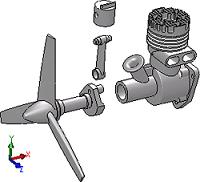
In this lesson, we provide more detail for carrying out the design problem of the single-piston engine (see Figure 1.18) discussed in Chapter 1. Recall in Section 1.5 that a cross-functional team was asked to develop a new model of the engine, with a 30% increment in both maximum torque and horsepower at the speed 1215 rpm. The design of the new engine was carried out at two interrelated levels: the system level and component level. At the system level, due to the increase in power and torque, the bore diameter of the engine case was increased from 1.416 to 1.6 in.; the crank length was increased from 0.5833 to 0.72 in.; and the connecting road length was increased from 2.25 to 2.49 in., as listed in Table 1.1. Also, the change causes the brake effective pressure Pb to increase from 140 to 180 lbf, causing peak combustion load increases from 400 to 600 lbf that act on the top face of the piston. The load magnitude and path applied to the major load-bearing components, such as the connecting rod and crankshaft, are therefore altered. Reaction forces applied to components, such as the connecting rod, increase. The increase in reaction forces raises concerns about the structural integrity of these load-bearing components in the engine. Changes may need to be made to strengthen the design of these components, which may cause an increase in manufacturing time and cost.
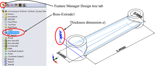
In Section 1.5, we discuss component-level design using the connecting rod as an example. We included structural analysis for stress, buckling load, and frequency, as well as machining time for the connecting rod. We parameterized the geometry of the connecting rod, and selected three dimensions: the diameter of the large hole (d32), the diameter of the small hole (d31), and the thickness (d7), as design variables (see Table 1.2). We carried out a sensitivity analysis for these structural performance measures and manufacturing time by varying these three design variables. We conducted design trade-offs and carried out a what-if study to come up with an improved design for the connecting rod.
In this lesson, we repeat the component-level design of the connecting rod using SolidWorks Motion, Simulation, and CAMWorks. We start with a motion model of the new design; that is, the changes in bore diameter, crankshaft length, and connecting rod length are made according to the new values shown in Table 1.1. We have prepared a structural model of the connecting rod with simulation results in static, frequency, buckling, and fatigue analyses. Also, a CAMWorks model is prepared. All are carried out for the new design; that is, the length of the connecting rod is 2.49 in. (increased from 2.25 in.). The objective of this lesson is to demonstrate the steps of conducting an interactive design process to achieve an improved design using the connecting rod example.
We start in Section S5.3.1 by describing the model files needed to carry out this exercise. We briefly describe the simulation results for the current design without showing the detailed steps in creating the models and running the simulations. Readers are encouraged to review tutorial projects S1–S4 for a good standing in solid modeling, motion analysis, structural analysis, and machining simulation, respectively, using SolidWorks CAD/CAE/CAM tools. With an understanding of the current design of the connecting rod, we move on to conduct sensitivity analysis in Section S5.3.2 and carry out a what-if study in Section S5.3.3. Note that some of the simulation results may not be consistent to those presented in Section 1.5, which were obtained using Mechanism, Pro/MECHANICA Structure, and Pro/MFG, with slightly different setups.
S5.3.1. Model Files and Current Design
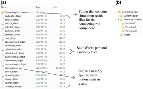
The example files downloaded from the book companion Web site should contain those shown in Figure S5.21(a) under the folder named “Project S5 Examples/Lesson S5.3 Single-Piston Engine.” The subfolder named “Connecting Rod” contains another three subfolders: Current Design, Sensitivity Analysis, and Whatif, as shown in Figure S5.21b. The “Current Design” folder contains simulation result files for the connecting rod at the current design, including static, frequency, buckling, and fatigue studies. Under “Sensitivity Analysis,” there are three subfolders: Perturb d7, Perturb d31, and Perturb d32. All are empty. We will store perturbed models and simulation results for the respective three design variables for sensitivity analysis using finite difference method. In the “Whatif” folder, there is a spreadsheet file (Whatif.xlsx) prepared for carrying out a what-if study.
In the following sections, we briefly go over the models and simulations for motion and structural analyses, as well as a machining simulation.
S5.3.1.1. Motion model and simulation
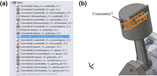
Start SolidWorks and open “Engine.sldasm” under the folder “Lesson S5.3 Single-Piston Engine.” You should see the engine assembly, as shown in Figure S5.22a. There are 21 assembly mates defined to create the motion model (see Figure S5.22a). One of them, Angle1, which is created to define the initial rotation angle of the spinner, is suppressed to provide the free degree of freedom. You may want to browse some of the assembly mates to gain a better understanding of the assembly and motion model, especially, “Concentric7” between the connecting rod and piston pin (see Figure S5.22b). This mate is chosen to monitor the reaction force acting on the connecting rod for structural analyses.
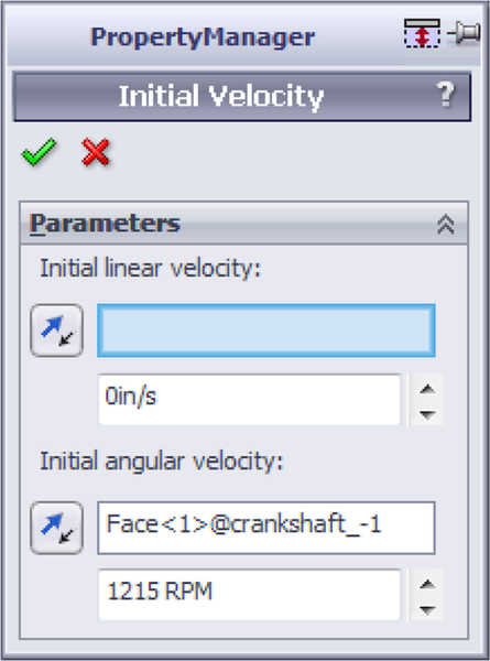
A motion simulation called “Motion Study” has been created. An initial angular velocity is defined and a force is applied to the piston at the beginning of the simulation. The initial velocity of 1215 rpm is defined on the crankshaft, as shown in Figure S5.23. A force of 600 lbf is applied to the top face of the piston for a short duration of 0.002 s, corresponding to about 6.5° of one rotation, as shown in Figure S5.24, to mimic the engine combustion force. Note that the force is applied only once at the beginning of the simulation, which is certainly not realistic. The combustion force cannot be applied to every single combustion cycle accurately due to the limitations of Motion capability.
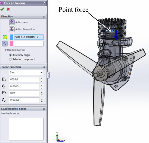
It will be more realistic if the force can be applied when the piston just starts moving downward (negative Y-direction) and can be applied only for a selected short period. In order to do so, we will have to define sensors that monitor the position of the piston for the combustion load to be activated. Unfortunately, such a capability is not available in Motion. Therefore, the force is simplified as a step function of 600 lbf along the negative Y-direction and applied for 0.002 s at the beginning of the simulation.
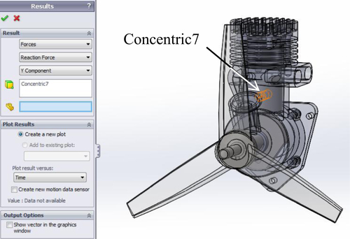
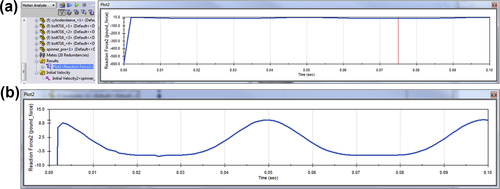
One result plot is created, which shows the reaction force at the upper joint of the connecting rod (Concentric7). The maximum reaction force is about −600 lbf at the beginning of the simulation. Click Results from the Motion Manager window to see an existing plot (Plot2<Reaction Force2>). Right-click Plot2 and choose Edit Feature to see the plot definition (Figure S5.25). Close the Results dialog box, right-click Plot2<Reaction Force2>, and then choose Show Plot. The graph of results appears as in Figure S5.26a. The reaction force due to inertia can be observed by zooming in the y-axis, in which the force reaches about 10 lbf, as shown in Figure S5.26b. For more information regarding the use of motion, readers are referred to Chang (2014b).
S5.3.1.2. FEA simulations
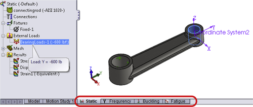
We now open the connecting rod model (connectingrod.SLDPRT) from the subfolder “Connecting Rod/Current Design.” Once open, you should see four (Simulation) design study tabs at the bottom of the graphics window—static, frequency, buckling, and fatigue, as shown in Figure S5.27. These are the simulations carried out for the current design. Click the Static tab, and choose External Loads > BearingLoads-1 to display the bearing load applied at the small hole of the rod. The inner face of the larger hole is fixed. Material used is AISI 1020. All simulation result files are included in the folder, so the results can be reviewed directly without rerunning the analysis.
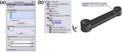
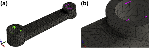
Click and expand Mesh to see mesh control. Right-click Control-1 to bring out the Mesh Control dialog box, as shown in Figure S5.28. As shown in the figure, a small region between the exterior surface of the small cylinder and the exterior surface of the rod was created for mesh refinement due to the high stress concentration found in the area. There are about 12,000 tetrahedron finite elements created for the rod with approximately 58,000 degrees of freedom. The mesh is shown in Figure S5.29.
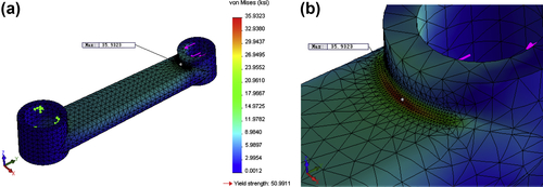
The static analysis results show that the maximum von Mises stress occurs in the area where mesh is refined, as shown in Figure S5.30. The stress is 35.93 ksi. The yield strength of AISI 1020 is approximately 51 ksi. The safety factor for current design is about 1.42.
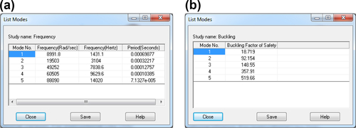
For frequency and buckling analyses, a fine mesh is chosen without any mesh control. The first five resonance frequencies and first five buckling loads are shown in Figures S5.31a and b, respectively. As shown in Figure S5.31a, the first (lowest) resonance frequency is 1431 Hz or 86,860 rpm, which is way higher than the operating frequency in the range of thousands rpm. Also, as shown in Figure S5.31b, the first (lowest) buckling load factor is 18.7, implying that the actual load that causes the connecting rod to buckle is 18.7 × 600 = 11,220 lbf, much higher than the firing load.
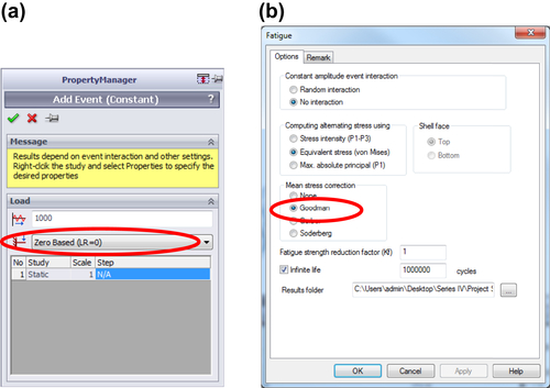
For fatigue analysis, we defined the 600 lbf load as a repeated load, where maximum is −600 lbf and minimum is 0 (very small inertia force in oscillation). Therefore, we choose the Zero Based (LR = 0) option (LR: load ratio), as shown in Figure S5.32a. Also, 1000 repetitions is defined as one block. Because the mean stress is nonzero, we choose the Goodman criterion for mean stress correction, as shown in Figure S5.32b. You may right-click “Fatigue” in the model tree and choose Properties to bring out the Fatigue dialog box of Figure S5.32b.
In addition, the S–N diagram and associated properties for AISI 1020 are shown in Figures S5.33a and b, respectively. Figure S5.33b appears by right-clicking the “connectingrod (-ASME Austenitic Steel-)” in the simulation model tree and choosing Apply/Edit Fatigue Data. In the Material dialog box, click View to show the S–N diagram in Figure S5.33a. The data in the Material dialog box shows that the endurance limit is about 29 ksi (corresponding to a fatigue cycle of 1,000,000).

Note that the stress in the static analysis is 35.9 ksi, which is greater than the endurance limit of the material. If the load (therefore, stress) is fully reversed, the fatigue life would have been about 2.3 × 10⁵, which can be estimated using the S–N diagram shown in Figure S5.33a.
The simulation results indicate that the fatigue life is infinite (>106) for the entire model because the stress is not fully reversed. For a more detailed discussion on fatigue analysis using Simulation, readers are referred to Project S3.4, which is part of Chang (2013a).
S5.3.1.3. CAMWorks machining
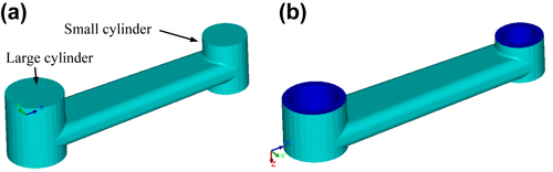
Manufacturing simulation was carried out using CAMWorks for the current design. We assume the machining operations start from a green part made by casting, as shown in Figure S5.34a. The machining operations remove materials on the top and bottom faces of the large and small cylinders, and drill two holes, as shown in Figure S5.34b.
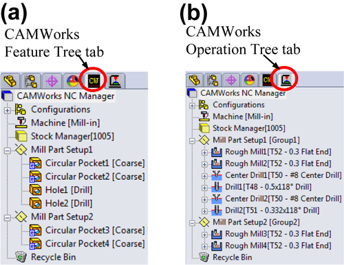
Entering CAMWorks from SolidWorks is straightforward. You may click the CAMWorks Feature Tree tab or Operation Tree tab to browse existing machining entities, as shown in Figure S5.35a and b.
If you do not see the CAMWorks pull-down menu, the CAMWorks Feature Tree tab, or the Operation Tree tab, you may have not activated the CAMWorks add-in module. To activate the CAMWorks module, choose from the pull-down menu:
In the Add-Ins dialog box, click CAMWorks in both boxes (Active Add-Ins and Start Up), and then click OK. You should see that CAMWorks is added to the pull-down menu.
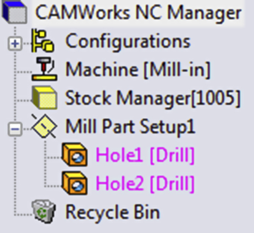
Click the Feature Tree tab. You should see that two mill part setups (Figure S5.35a), Mill Part Setup1 and Mill Part Setup2, are included for machining the faces on both sides of the connecting rod. Mill Part Setup1 consists of four machinable features: Circular Pocket1, Circular Pocket2, Hole1, and Hole2 and Mill Part Setup2 has two features, Circular Pocket3 and Circular Pocket4, as shown in Figure S5.35a.
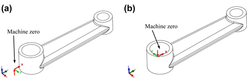
Click the Operation Tree tab to see the eight machining operations created under Mill Part Setup1 and Mill Part Setup2, as shown in Figure S5.35b. Note that each Rough Mill operation is for machining a circular surface, whereas each hole feature will result in a center drill operation plus a follow-on hole-drilling operation. The machine zeroes for the respective setups are shown in Figures S5.36a and b. Note that the Z-axis of the machine zero of Setup1 is pointing in the negative Z-axis of the world coordinate system. For Setup2, the Z-axis is in parallel with that of the world coordinate system. In practice, jigs and fixtures must be designed and fabricated to hold the green part in support of the machining operations at shop floor. The machine zeroes may need to be adjusted according to the fixture design.
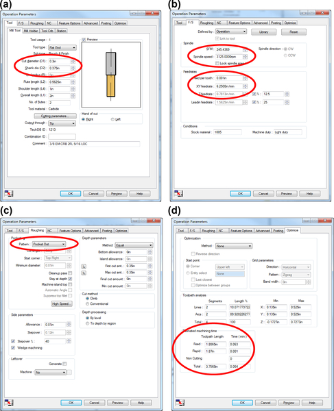
Right-click Rough Mill1 (under Mill Part Setup1) and choose Edit Definition; the Operation Parameters dialog box appears. A 3/8 EM CRB 2FL flat end cutter is chosen for all Rough Mill operations, as shown in Figure S5.37a. The machining parameters, such as spindle speed and feed per tooth, generated from CAMWorks database are under the F/S tab, as shown in Figure S5.37b. Setups for the roughing operations are under Roughing tab, as shown in Figure S5.37c. The machining time, such as Rough Mill1, which removes a thin-layer material on the bottom face of the large cylinder, is given in the Optimize tab shown in Figure S5.37d (in this case, 0.381 min). Note that this includes only the actual machining time when the cutter is in motion. Setup time, tool change time, and so forth are not included.
Note that instead of using default values, we modify the machining parameters as follows: for rough mill, feed per tooth changed from 0.006 to 0.001 in.; for center drill, the Z feed rate changed from 6 to 2 in./min; and for hole-drilling, the Z feed rate changed from 8 to 1 in./min.
You may see the complete machining operations by choosing the following from the pull-down menu:
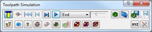
CAMWorks > Simulate Toolpath
Then, click the Run key (▸) in the Toolpath Simulation dialog box (Figure S5.38) to play the toolpath simulation.
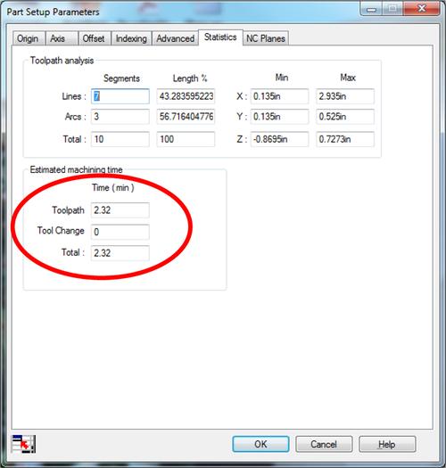
The overall machining time can be found by right-clicking the mill part setup, such as Mill Part Setup1, and choosing Edit Definition. In the Part Setup Parameters dialog box (Figure S5.39), choose the Statistics tab to see the machining time for the entire setup. The machining times for Setup1 and Setup2 are 2.32 and 1.81 min, respectively. Total is 4.13 min. You may easily double-check these numbers by adding the times from individual operations. For example, for Setup1, we add the machining times of the six individual operations as 0.381 + 0.206 + 0.238 + 0.768 + 0.166 + 0.567 = 2.326 min, which is the same as the time obtained from Setup1.
A brief description of the construction of the machining model can be found in Appendix A. More detailed discussion on CAMWorks can also be found in Project S4 of Chang (2013b).
S5.3.2. Sensitivity Analysis
The three design variables defined for the connecting rod are the diameter of the larger hole (d32), diameter of the small hole (d31), and the thickness (d7). For the current design, the values of the design variables are, respectively, d32 = 0.5 in., d31 = 0.334 in., and d7 = 0.25 in.
To carry out sensitivity analysis for the gradients of the performance measures, including von Mises stress, lowest resonance frequency, lowest buckling load, fatigue life, volume, and machining time with respect to the three design variables, we use the overall finite difference method discussed in Chapter 3.
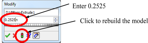
The approach is very simple. We perturb the individual design variables, one at a time, by 1% of its design variable value. For example, we change the thickness d7 from 0.25 to 0.2525 in., regenerate the model, and then carry out simulations to find the values of the performance measures at the perturbed design. Thereafter, the sensitivity of a performance ψ(x) can be approximated as:
![]() (S5.3)
(S5.3)
where ψ(x + Δx) is a performance measure value obtained at the perturbed design from simulation, and Δx is the design perturbation (e.g., Δd7 = 0.0025 in.).
The detailed steps are described next. We copy the SolidWorks part file connectingrod.SLDPRT from the folder “Connecting Rod/Current Design” and paste it to folders “Connecting Rod/Sensitivity Analysis/Perturb d7,” “Perturb d31,” and “Perturb d32,” respectively.
Then, from SolidWorks we open connectingrod.SLDPRT in folder “Connecting Rod/Sensitivity Analysis/Perturb d7,” click the Feature Manager Design tree tab to display the model tree, and double-click the Boss-Extrude1 feature to display the thickness dimension d7, as shown in Figure S5.40.
Double-click the thickness dimension, enter the perturbed dimension value 0.2525 in., and click the Regenerate button (see Figure S5.41) to rebuild the model.
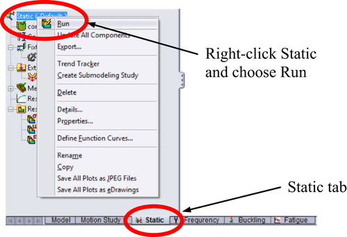
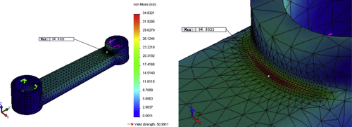
Click the Static tab below the graphics window, and right-click Static in the model tree to choose Run (see Figure S5.42). After the simulation is completed (in a short period), double-click Results and Stress1 to show the stress fringe plot, as shown in Figure S5.43. The fringe plot shows that the maximum von Mises stress becomes 34.83 ksi and is located in approximately the same location as the original design because the perturbation in design variables is small. This value is plugged into Eq. S5.3 to calculate the gradient:
![]()
We repeat the same steps to rerun simulations for frequency, buckling, and fatigue. The results are shown in Figure S5.44.
Note that volume of the connecting rod can be obtained by choosing from the pull-down menu:
Volume and other mass properties are shown in the Mass Properties dialog box, as shown in Figure S5.45. Note that by default, only two or three digits are shown, which may cause a loss of significant digits when calculating the gradients. You may increase the number of digits by choosing from the pull-down menu:
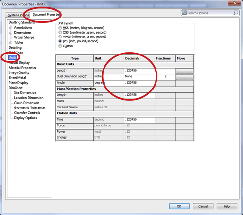
Tools > Options.
In the Document Properties dialog box (Figure S5.46), choose the Document Properties tab, and click Units. Pull down a data field, such as Length under Decimals (see Figure S5.46) and choose, for example, 123456 to increase the number of digits to 6.
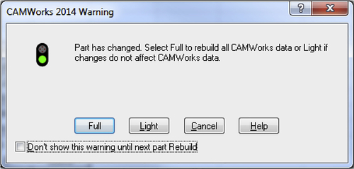
Now, we rerun the machining simulation. Click the Model tab below, and choose the CAMWorks Operation Tree tab above the model tree to get back to CAMWorks. Because the model is perturbed, a warning message appears (see Figure S5.47). In the CAMWorks 2014 Warning dialog box, we click Full to update CAMWorks data.
Update the toolpath by choosing from the pull-down menu:
CAMWorks > Generate Toolpath
After regenerating the toolpath, the machining time can be found by choosing Edit Definition from setups or individual operations, as discussed before. Note that the machining times are unchanged because the change in the thickness design variable d7 is not affecting the machining operations, which remove materials at the top and bottom faces of the two cylinders and drill two holes for the respective cylinders. Therefore, sensitivity of the machining time with respect to the thickness design variable is zero.
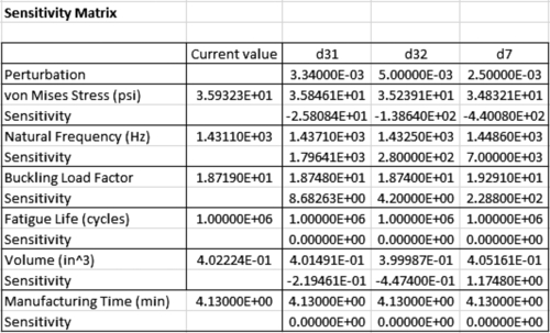
We repeat the steps discussed earlier for design variables d31 and d32, by changing them to d32 = 0.505 in. and d31 = 0.33734 in. We carry out simulations and toolpath generations for the two perturbed designs. The sensitivity matrix for the three design variables are calculated as shown in Figure S5.44.
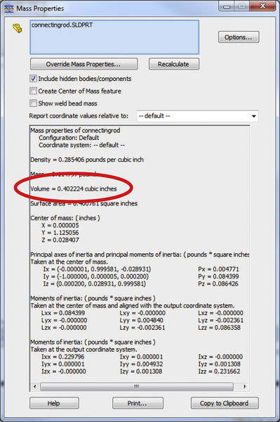
In Figure S5.44, the sensitivity coefficients of the machining time for all three design variables are zero because the design perturbations did not affect the machining operations. Although the hole sizes are changed, we assume the use of drill bits of the same sizes as the holes; therefore, toolpath and machining time are unchanged. Also, the sensitivity coefficients of the fatigue life are all zero because the fatigue life is infinite before and after design perturbations. Moreover, some of the coefficients may not have enough significant digits. For example, if only four digits were chosen in the Document Properties dialog box, the volume sensitivity of design variable d31 is calculated in spreadsheet as 2.70915E–05. In fact, the difference of volume before and after design perturbation is 0.4022 − 0.4015 = 0.0007—only one significant digit. In order to increase the accuracy of the volume sensitivity coefficients, we need more digits. We did choose six decimals earlier in the Document Properties dialog box, so we should have enough significant digits. For performance measures, such as the resonance frequency, there may not be a way to increase the number of digits without extracting data from SolidWorks database via application protocol interface.
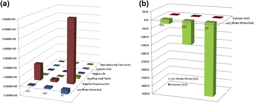
A bar chart of the entire sensitivity coefficient matrix (6 × 3 in this case) can be created using Spreadsheet, as shown in Figure S5.48a. The bar chart provides a global view on the influence of individual design variable to all performance measures and all design variables to a single performance measure. For example, natural frequency increases by increasing any of the three design variables. Among them, d7 is the most significant and d32 is the least effective. Increasing design variable d7 decreases stress, increases natural frequency, increases buckling load, and so on. Because the sensitivity magnitudes of different measures are different (by an order of magnitude), a common practice is normalizing these gradients by their respective maximum values for a better comparison of the effect of one variable across performance measures.
If we want to reduce stress and not increase volume much, we may graph the sensitivity coefficients for these two performance measures only, as can be seen in Figure S5.48b. The bar chart shows that the von Mises stress is reduced by increasing any of the three design variables. Among them, d7 is the most significant and d31 is the least influencing. On the other hand, only a small change in volume is observed.
S5.3.3. What-If Study
We go over a what-if study for the goal of reducing von Mises stress and not increasing volume too much. As seen in the bar chart in Figure S5.48b, we increase all three design variables by using the steepest decent direction of the stress measure. As discussed in Chapter 3, the steepest decent direction of the stress measure is defined as:
 (S5.4)
We then use a small step size, for example α = 0.01, and multiply it by the normalized vector n for design perturbations:
![]() (S5.5)
(S5.5)
The design perturbation δx is shown in the cells C29 to E29 of the “Whatif” spreadsheet, as shown in Figure S5.49. The current and predicted performance measure values are listed in Cells F22 to G27, and the percentage changes between them are shown in Cells H22 to H27. The cells indicate that the changes are below 13%, which are acceptable. The stress is reduced by about 13%, with only a 2% increase in volume. The design seems to be desirable.
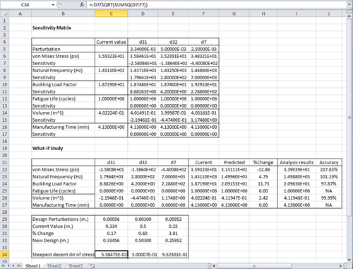
To carry out simulation of the new design, we first copy the SolidWorks model of the current design (located in folder: “Connecting Rod/Current Design”) and paste it to folder “Connecting Rod/Whatif.” We then open this model from SolidWorks and update the solid model by entering the new design variables: d31 = 0.33456, d32 = 0.50300, and d7 = 0.25952. We regenerate the solid model and rerun the simulations. The simulation results are entered into the spreadsheet (Cells I22 to I27); the accuracy of the prediction and analysis results are shown in Cells J22 to J27. The predictions are accurate except for stress. This could be caused by either insufficient accuracy of the sensitivity or design perturbations that are not small enough.
In any case, the design is improved with the maximum von Mises stress reduced from 35.93 to 33.90 ksi and small increase in volume (0.4022 to 0.4119 in.3). The process discussed above can be repeated if needed. For the time being, we are satisfied with the design and will stop here.
Appendix A. Creating the Machining Model in CAMWorks
In this appendix, we briefly discuss the key steps in creating the machining model of the connecting rod in CAMWorks. We assume readers are familiar with CAMWorks. If not, readers are referred to Project S4 of Chang (2013b) for more information before going over the discussion in this appendix.
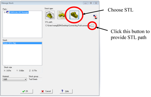
First, the workpiece employed is an STL (stereolithography) model. To bring in an STL model as a workpiece, we first choose the CAMWorks Operation Tree tab, right-click Stock Manager, and choose Edit Definition. In the Stock Manager dialog box (Figure A.1), choose STL and click the button next to the STL path to choose the STL model and bring it in. The workpiece should appear in the graphics window.
Only the two holes are recognized automatically using Extract Machinable Features (pull-down menu: CAMWorks > Extract Machinable Features). Once extracted, they are listed under Mill Part Setup1, as shown in Figure A.2. There is no need to do anything else. The toolpath of the center drill and follow-on hole-drilling operations can be generated automatically.
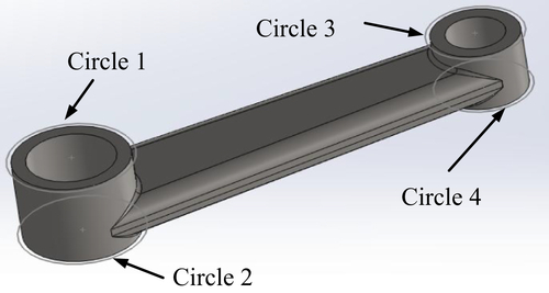
Machining features for the rough mills that remove materials on the top and bottom faces of the two cylinders cannot be extracted automatically. Sketches need to be created. Four circles are sketched, as shown in Figure A.3. The diameter of each circle is 0.05 in. larger than that of the circular edge on the respective cylinders.
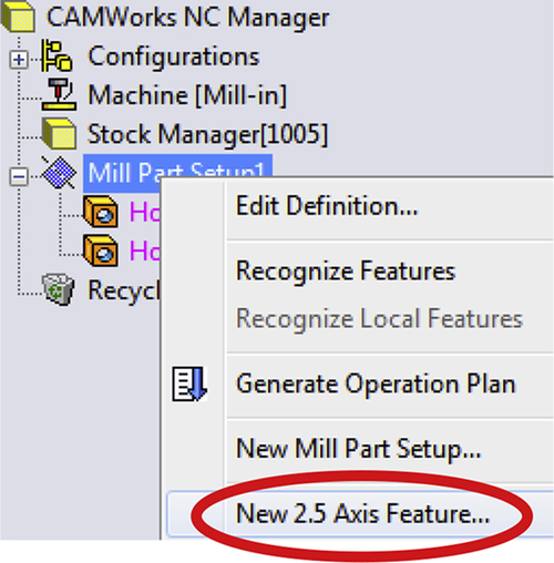
Then, we create machining features manually by selecting the circles or sketches. First, right-click Mill Part Setup1 and choose New 2.5 Axis Feature (see Figure A.4). In the 2.5 Axis Feature Wizard (see Figure A.5), select feature type Pocket, click Multiple, and then choose Circle 2 and Circle 4 in the graphics window (flip the model in the graphics window to pick the two circles). Or, simply click Sketch6 under the Use column. Click Next.
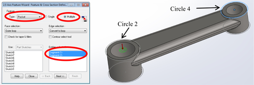
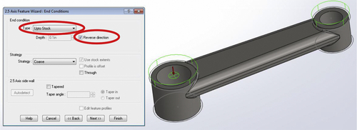
Choose upto Stock as End Condition, click Reverse direction (default), and then click Next and Finish (see Figure A.6). Close the wizard. Two newly created circular pockets (Circular Pocket1 and Circular Pocket2) are listed under Mill Part Setup1.
Next, we create another mill part setup (because part needs to be flipped before the other two faces can be machined).
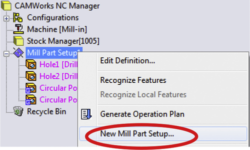
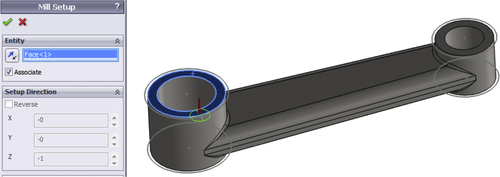
Right-click Mill Part Setup1 and choose New Mill Part Setup (see Figure A.7). Rotate the model in the graphics window (if needed) and pick Face<1> as the plane to define Z-axis of machine zero, as shown in Figure A.8. Use the default machine zero.
Like before, we manually create machining features by selecting the remaining two circles (Circles 1 and 3).
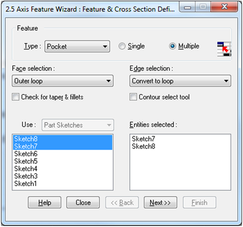
First, right-click Mill Part Setup2 and choose New 2.5 Axis Feature. In the 2.5 Axis Feature Wizard (see Figure A.9), select feature type Pocket, click Multiple, and then choose Sketches 7 and 8 under the Use column. Click Next.
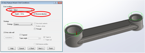
Choose Blind, click Reverse direction (default), and enter 0.1 in. for End Condition, and then click Next and Finish (see Figure A.10). Close the wizard. Two newly created circular pockets are listed under Mill Part Setup2.
At this point, you should be able to generate a toolpath by choosing Generate Operation Plan and Generate Toolpath from the CAMWorks pull-down menu.
Questions and Exercises
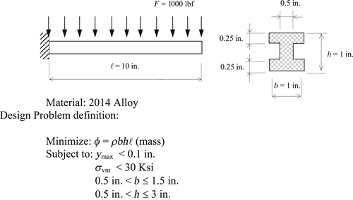
S5.1 Design the following cantilever beam using optimization capability in SolidWorks Simulation.
a. Create SolidWorks and Simulation models, and carry out optimization. Submit screen captures for the stress and displacement at the initial and optimal designs found by SolidWorks Simulation. Submit design history graphs for objective, constraints, and design variables.
b. Solve the same problem by adjusting the two design variables manually. Is your design better than that of SolidWorks Simulation? If so, by how much (e.g., mass %)? Submit screen captures for the stress and displacement at the improved design.
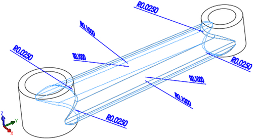
S5.2 Carry out sensitivity analysis and at least one what-if study for the connecting rod, following steps similar to that of Section S5.3. In this exercise, we use the same performance measures and three design variables: thickness (d7, same as that of Section S5.3), and the two groups of fillets shown in the figure above. That is, fillets of radius R 0.1 in. and fillets of radius R 0.025 in. Use plain carbon steel as the material (yield strength: 32 ksi and endurance limit 30.5 ksi). When calculating the fatigue life, we assume the load is fully reversed (hence, choose load ratio LR = −1). The final design must be feasible; that is, maximum von Mises stress must be less than the yield strength divided by a safety factor of 1.2, fatigue life must be infinite, resonance frequency must be greater than the operating frequency (2000 rpm), and buckling load factor must be greater than the firing load of 600 lbf with a safety factor 1.2. Report the following findings:
a. Simulation results for the current design, including maximum von Mises stress, frequency, buckling load, fatigue life, and volume. Is the current design feasible? If not, identify the performance measures that are over the limits (with safety factors considered).
b. Sensitivity matrix, including how you perturbed the three design variables; for example, is 1% perturbation adequate for all three design variables?
c. Report how you came up with a feasible design.
d. Describe how you can continue to reduce the volume of the connecting rod once you are in the feasible region, if possible.
..................Content has been hidden....................
You can't read the all page of ebook, please click here login for view all page.