
3.11. Tutorial Example: Simple Cantilever Beam
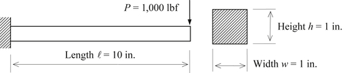
We use the cantilever beam example shown in Figure 3.4 to illustrate detailed steps for carrying out design optimization using SolidWorks Simulation and Pro/MECHANICA Structure. The beam is shown in Figure 3.46 again with a few more details. The beam is made of aluminum (2014 Alloy) with modulus of elasticity E = 1.06 × 10⁷ psi and Poisson's ratio υ = 0.33. At the current design, the beam length is ℓ = 10 in., and the width and height of the cross-section are both 1 in. The load is P = 1000 lbf acting at the tip of the beam, as shown in Figure 3.46. Our goal is to optimize the beam design for a minimum volume subject to displacement and stress constraints by varying its length as well as the width and height of the cross-section.
The design problem of the cantilever beam example is formulated mathematically as
![]() (3.100a)
(3.100a)
![]() (3.100b)
(3.100b)
![]() (3.100c)
(3.100c)
![]() (3.100d)
(3.100d)
in which σmp is the maximum principal stress, and δy is the maximum displacement in the y-direction (vertical).
This design problem will be implemented and solved using both Simulation and Mechanica in Projects S1 and P1, respectively. We briefly discuss the example in this section. Detailed step-by-step operations in using the software tools can be referred to the respective projects.
3.11.1. Using SolidWorks Simulation
SolidWorks Simulation employs a generative method for support of design optimization. Design variables are varying between their respective lower and upper bounds. These design variables are combined to create individual design scenarios. Finite element analyses are carried out for all scenarios generated. Among the scenarios evaluated, feasible designs are collected; and within the feasible designs, the best design that yields the lowest value in the objective function is identified as the solution to the design problem.
In the beam example, we chose a 0.5 in. interval for varying the width and height design variables, and a 5 in. interval for the length design variable. As a result, each design variable is varied three times. For example, the width design variable is changed from its lower bound of 0.5 in. to 1.0 in., and then to its upper bound 1.5 in. Similarly, three changes take place for the height and length design variables, respectively. These changes in design variables are combined to create 27 (3 × 3 × 3) scenarios to search for an optimal solution.

A static design study is created for the beam with boundary and load conditions shown in Figure 3.47. Also shown in Figure 3.47 are the finite element mesh (default median mesh) and the fringe plot of the maximum principal stress (or first principal stress).
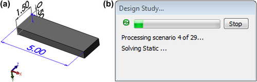
A total of 29 static analyses (27 plus initial and current designs) will be carried out for the study. In the graphics window, the designs of all scenarios will appear in the beam with changing dimensions, as shown in Figure 3.48.
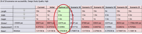
At the end, an optimal solution is found for Scenario 19 (see Figure 3.49), in which width, height, and length become 0.5, 5, and 1.5 in., respectively. Displacement is 0.0296 in. (<0.1 in.), stress is 42,076 psi (<65 ksi), and the total mass is 0.379 lb (reduced from 1.01 lb from initial design).
3.11.2. Using Pro/MECHANICA Structure
Unlike Simulation, Mechanica employs a gradient-based solution technique for solving design problems. Accessing the optimization capability in Mechanica is similar to that of defining and solving an FEA, which is straightforward.
A static design study is created for the beam with boundary and load conditions shown in Figure 3.50a. Figure 3.50a also shows the finite element mesh (13 tetrahedron solid elements). The maximum bending stress fringe plot is shown in Figure 3.50b, which shows maximum tensile and compressive stresses, respectively, at the top and bottom fibers of the beam close to the root end. FEA results are also given in the status dialog box shown in Figure 3.50c, in which maximum displacement and principal stress are 0.373 in. and 71.92 ksi, respectively.
An optimal solution is obtained in seven design iterations. At the optimum, the three design variables are length ℓ = 5 in., width w = 0.5 in., and height h = 1.08 in. Constraint functions are stress σmp = 64.99 ksi, and displacement δx = 0.0766 in.; both are feasible. The total mass is 0.0007056 lbf s2/in. (or 0.272 lbm), reduced from 0.002669 lbf s2/in. (or 1.03 lbm) from the initial design. The optimization history graphs for objective and constraint functions are shown in Figures 3.51a, b, and c, respectively.
..................Content has been hidden....................
You can't read the all page of ebook, please click here login for view all page.