Chapter 2. Assembly Language
For the things we have to learn before we can do them, we learn by doing them.
—Aristotle, Nichomachean Ethics
This chapter is about writing assembly-language software. This is a difficult subject to present, as it is a very diverse topic. There are many processors covered in this book. The assembly language of one processor bears no relation to that of another. To delve into the assembly language of each would require an entire book in its own right (or several books). Hence, I’m not even going to attempt to cover each one’s instruction set. Instead, I’m going to concentrate on just two processors, the 68HC11 and the PIC, and use these as vehicles to show you some basic assembly- language techniques. I’m not going to dissect the instruction sets in detail. The User’s Manual/datasheets for the processors give full descriptions of the instructions and their operation.
Assembly-language programming works down at the machine level, and as such, you really get a feel for what the processor is doing and how your computer actually works. While assembly-language programming can be fun, it can also be a daunting task to code major applications in it. To this end, assembly is usually used in only two instances. The first is for the development of simple test software during the early prototype development of a system. Such software may simply initialize the machine to a known state and perform some simple task such as flashing a LED or outputting the venerable “hello world” to a terminal or host.
With assembly language, you work with data in single bytes or words at a time. Processors store data within memory, and this is usually implemented using external chips in the computer system. To manipulate data, processors use registers within the CPU.
No computer can understand assembly directly. Back in the olden days, when computers were steam-driven and tended by gnomes, software was compiled manually. Each instruction mnemonic was looked up and converted to the appropriate opcode by the programmer. While it is certainly character-building, converting from assembly to opcodes is very tiresome, particularly where large programs are concerned. To make life easier, special compilers, called assemblers , take mnemonics and convert them to opcodes.
Assembly language has been described as the “nuts and bolts language,” because you are writing code directly for the processor. For a lot of the software you will write, a high-level language like C will be the language of choice. High-level languages make developing software much easier, and your code is also portable (to a degree) between different target machines. Compilers of high-level languages convert your source code down to machine opcodes. Thus, by using a compiler, the programmer is relieved of having to know the specific details of the processor, and of having to code his program directly in machine code.
So there are good reasons for using a high-level language, yet programmers often write directly in assembly language. Why? Assembly and machine code, because they are “hand-written,” can be finely tuned to get optimum performance out of the processor and computer hardware. This can be particularly important when dealing with time-critical operations with I/O devices. Further, coding directly in assembly can sometimes (but not always) result in a smaller code space. So, if you’re trying to cram complex software into a small amount of memory and need that software to execute quickly and efficiently, assembly language may be your best (and only) choice. The drawback, of course, is that the software is harder to maintain and has zero portability to other processors. A good software engineer can create more efficient code than the average optimizing C compiler; however, a good optimizing compiler will probably produce tighter code than a mediocre assembly-language software engineer. Typically, you can include in-line assembly within your C code, and thereby get the best of both worlds.
At the mere mention of assembly language, many a die-hard programmer begins to quiver in fear, as if just invited into a tiger’s cage. However, assembly-language programming is not that hard and can often be a lot of fun. Think of it as being “as one” with the processor.
That said, this is a book predominantly about hardware, not software. In this chapter, we’ll take a quick tour of assembly-language programming, just to give you an overview. In the next chapter, we’ll take a look at the Forth programming language, widely used in many embedded systems. For more information on embedded software development, I highly recommend two O’Reilly books: Programming Embedded Systems by Michael Barr and Anthony Massa, and Programming with GNU Software by Mike Loukides and Andy Oram. If you want to build a Linux-based embedded computer, I recommend Building Embedded Linux Systems by Karim Yaghmour, also published by O’Reilly.
Let’s start by looking at the internal storage of the processor.
Registers
Registers are the internal (working) storage for the processor. The number of registers varies significantly among processor architectures. Typically, the processor will have one or more accumulators . These are registers that may have arithmetic operations performed on them. In some architectures, all the registers function as accumulators, whereas in others, some registers are dedicated for storage only and have limited functionality.
Some processors have index registers that can function as pointers into the memory space. In some architectures, all general-purpose registers can act as index registers; in others, dedicated index registers exist.
All processors have a program counter (also known as an instruction pointer ) that tracks the location in memory of the next instruction to be fetched and executed. All processors have a status register (also known as a condition-code register, or CCR ) that consists of various status bits (flags) that reflect the current operational state. Such flags might indicate whether the result of the last operation was zero or negative, whether a carry occurred, if an interrupt is being serviced, etc.
Some processors also have one or more control registers consisting of configuration bits that affect processor operation and the operating modes of various internal subsystems. Many peripherals also have registers that control their operation and registers that contain the results of operations. These peripheral registers are normally mapped into the address space of the processor.
Some processors have banks of shadow registers , which save the state of the main registers when the processor begins servicing an interrupt. By using shadow registers, there is no need to save processor state to the stack. This can save significant time in servicing an interrupt. (We’ll look at stack operations in more detail shortly.)
Processors are commonly 8-bit, 16-bit, 32-bit, or 64-bit, referring to the width of their registers. An 8-bit processor is invariably low-cost and is suitable for relatively simple control and monitoring applications. If more processing power is required, the larger processors are preferable, although cost and system complexity increase accordingly.
Machine Code
Everything that a processor deals with is expressed as numbers in memory. That applies to data, and to software as well. Your compiled C program is converted to a sequence of numbers that is meaningful to the processor as a sequence of instructions. A program that a processor (in this case, a 68HC11) can execute might look something like:
86 41 B7 01 00 BD 02 00
This is known as machine code, and each numeric instruction is called an opcode. Humans find such programs very hard to write and even harder to understand. To make this easier to cope with, we use a notation called assembly language. Assemblylanguage instructions equate directly to their machine code counterparts. Since machine code is difficult to read and write (for a human), a mnemonic is used to represent the opcode. For example, the 68HC11 instruction 86 41 is more easily understood by its mnemonic LDAA #$41. (The dollar sign [$] represents a hex value in some assembly languages.) This is still a bit cryptic, so we usually add comments on the righthand side to help us follow what is going on. The previous machine code sequence written as 68HC11 assembly would be:
Machine code   Assembly    Comment
86 41          LDAA #$41   ; anything after a semi-colon
B7 01 00       STAA $0100  ; is a comment
BD 02 00       JSR $0200   ;
LDAA #$41 means “load accumulator A with the immediate value (signified by the #) of 0x41.”
Immediate
means that the operand is to be treated as a number, rather than as a pointer to an address. With some processors, this is known as a literal. LDAA corresponds to the machine opcode 86.
STAA $0100 tells the processor to store the contents of accumulator A to the memory location (no # this time) 0x0100.
JSR $0200 means “jump to the subroutine at address 0x0200.” A subroutine is essentially a procedure or function call. In some processors, the instruction to do this is call, rather than jump.
The instructions of a Freescale Semiconductor 68HC11 series processor (Chapter 16) can be from one to three bytes in length. The first byte is always an opcode and may be followed by one or two bytes of data. For example, consider the following assembly-language program:
Machine code   Assembly    Comment
CE 10 02       LDX #$1002  ; load index register X with 0x1002
5F             CLRB        ; clear accumulator B
86 41          LDAA  #$41  ; load accumulator A with 0x41.
Note the length of each instruction. The first instruction takes three bytes, the second takes only one, and the third is two bytes in length. The number of bytes an instruction takes depends on what it does. This is true for CISC processors, but not RISC. In order to achieve simpler instruction decode units, RISC processors have instructions of a fixed size, with operands buried inside the instruction. For example, all instructions of a PIC16 processor are 14 bits wide, regardless of what operation they perform.
Different processors use different assemblies. No two are alike. The previous examples are written in 68HC11 assembly. This assembly is applicable only to the 6800 family of processors, of which the 68HC11 is a member. Other assembly languages, because they are based on very different processor hardware, have very different syntax. Some examples of different versions of the same operation are given in Table 2-1. In each case, a register is loaded with a byte value of 0x41. (Note also the different ways of expressing hex notation.)
Signed Numbers
Before getting into the nuts and bolts of assembly, let’s take a quick look at how signed numbers are represented within the machine. Negative and positive numbers can be represented in binary (or hex) number systems by the state of the most significant bit. If the most significant bit is set, this indicates that the number is negative.
Tip
It is up to the programmer whether to treat the content of a register or memory location as signed or unsigned. In C, we are used to explicitly declaring a variable or pointer as either signed or unsigned. In assembly, it’s up to you.
An 8-bit accumulator can have (in decimal) 0 to 255 (unsigned) or -128 to +127 (signed). Given a positive number, we use two’s complement to convert this to its negative equivalent. Taking the two’s complement of a number is done by inverting the bits (a one’s compliment) and adding one to the result. So 0xFF is 1111 1111 (in binary) and is therefore negative. 0xFF is used to represent -1, 0xFE is -2, etc., all the way to 0x80, which is -128 (decimal).
For example, -3 as an 8-bit hex value is calculated in this way:
             0 0 0 0   0 0 1 1  (0x03)
Invert bits: 1 1 1 1   1 1 0 0  (0xFC)
Add 1 gives: 1 1 1 1   1 1 0 1  (0xFD)
So -3 is 0xFD in hex.
Note that we are not limited to using signed (positive and negative) numbers. We are free to ignore the sign bit and treat the byte as an unsigned number, giving us a range of 0x00 to 0xFF (255 decimal). It all depends on what we want the byte to represent.
16-bit, 32-bit, and 64-bit signed numbers work in the same way. The most significant bit represents the sign, and the remaining bits constitute the number.
Addressing Modes
The different ways in which an instruction can reference a register or memory location are known as the addressing modes of the processor. The types of addressing modes available within different architectures vary. To illustrate some of the more common modes, let’s take a look at those available in the 68HC11 architecture:
- Inherent
The instruction deals purely with registers.
CLRBclears the B accumulator, for example.- Immediate/Literal
The instruction has a literal number as an operand.
- Direct
The instruction accesses a memory location, specified by a short address. In other words, direct addressing provides access to a subset of the total address space. On a given processor with a 16-bit address bus, a direct access may, for example, specify an address within the first 256 bytes. On a 32-bit processor, a direct access may specify an address within the first 64K of memory, for example. Direct addressing is used (when possible) to reduce the length of instruction-referencing memory. This can reduce code size, and therefore instruction fetch time, in time-critical applications. Many processors, especially RISC, do not use direct addressing.
- Extended
The instruction accesses a memory location, specified by the full address. So
LDAA $B098means load accumulator A with the contents of address0xB098in memory.- Indexed
The instruction uses the contents of a register as a pointer into memory. If, for example, the X register is equal to
0x5034, thenLDAA 0,Xmeans “load accumulator A with the contents of the location pointed to by X.” In this example, this means “load accumulator A with the contents of address0x5034.” WhereasLDAA 2,Xmeans “load accumulator A with the contents of the memory location pointed to by X, but with an offset of 2.” So if X =0x5034, then2,Xis0x5036.SoLDAA 2,Xloads from address0x5036. Indexed addressing is useful when your program needs to reference data in a table or list. The index is an easy way of moving through the data structure.- Relative
An offset is specified as part of the addressing. A branch instruction uses relative addressing to add (or subtract) a value from the program counter. For example,
bra 02(branch) adds 2 to the program counter, whereasbra $FFadds -1 to the program counter. Note that the instruction counter always points to the next instruction, not the one currently being executed.
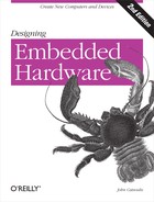
Big-Endian and Little-Endian Addressing
Microprocessors are either big endian or little endian in their architecture. This refers to the way in which the processor stores data (16 bits or greater) to memory. A big-endian
processor stores the most significant byte at the least significant address, as illustrated in Figure 2-1. In each case, the data has been stored to address 0x0100.

A little-endian processor stores the most significant byte at the most significant address, as shown in Figure 2-2.
With the little-endian scheme, the least significant data travels over the least significant part of the data bus and is stored at the least significant memory location. For a programmer, it is conceptually easier to understand in terms of data path. The inconvenience of little endian is that data appears “backwards” in the computer’s memory if you display a block of locations. Storing the value 0x12345678 to memory results in 0x78563412 in the memory space. Note that a little-endian processor will read this data back correctly; it’s just that it makes it harder to understand the numbers if a human is looking at the memory directly. Alternatively, a big-endian processor storing 0x12345678 to memory results in 0x12345678 sitting inside the memory chip. This appears (to a human) to make more sense. Neither scheme has much advantage over the other in terms of operation; they are just two different ways of doing the same thing. When you’re doing high-level programming on a system, the “endian-ness” makes little difference. The only time you are really exposed to it is when you are dealing with multibyte data and accessing it on a byte-by-byte basis. However, when you are developing and debugging hardware and low-level firmware, you come across it all the time, and so an understanding of big endian and little endian is important.
Coding in Assembly
Assembly-language programming is not difficult, particularly with the smaller microcontroller and microprocessor architectures. The main difficulty many people seem to have is knowing how to tackle a given programming problem. As with any other language, there are always many ways in which a program may be written. There is rarely a single “right way” (although there may be a “most efficient way”). It is simply a matter of breaking down the problem into a series of tiny steps.
For example, let’s say we want a 68HC11 processor to add three numbers together (0x10, 0x1F, and 0x0C) and store the result at address 0x0027. This problem is easily broken down into four steps. We take the first number (step one), add the second number (step two), add the third number (step three), and store the result (step four). We want to do some arithmetic, so we choose an accumulator to hold our numbers, since accumulators
are registers designed for this type of operation. We start by loading an accumulator with the first number:
LDAA #$10 ; load first number into the A accumulator
The A accumulator now contains the number 0x10 (16 in decimal). Remember that the "#" in the instruction means that the addressing mode is immediate. In other words, the processor is to load the actual number 0x10, not use the operand as a pointer. We then want to add the number 0x1F. So our next instruction is:
ADDA #$1F ; add the second number to the A accumulator
This causes 0x1F to be added to accumulator A. Again note the "#.” Similarly, to add the third number, we have:
ADDA #$0C ; add the third number to the A accumulator
Finally, we store the result at address 0x0027:
STAA $0027 ; store the contents of the A accumulator to address 0x0027
This time, note that there is no "#.” This is an extended instruction. It means “Store the contents of accumulator A to the memory location 0x0027.” It does not treat 0x0027 as a number, but rather as the address of a location in memory.
So our complete program is:
LDAA   #$10   ; load first number in the A accumulator
ADDA   #$1F   ; add the second number to the A accumulator
ADDA   #$0C   ; add the third number to the A accumulator
STAA   $0027  ; store the contents of the A accumulator to address 0x0027
To make this program into a subroutine (a callable function or procedure), we simply add a label at the start and a return-from-subroutine (RTS) instruction at the end. (We’ll look at subroutines in more detail shortly.) A label is used by the assembler during compilation to identify a given address location. It has no direct meaning in the machine code:
add_numbers
   LDAA   #$10   ; load first number in the A accumulator
   ADDA   #$1F   ; add the second number to A
   ADDA   #$0C   ; add the third number to A
   STAA   $0027  ; store the contents of A to address 0x0027
   RTS           ; return to main program
To call our subroutine from our main program, we simply use a jump-to-subroutine instruction (JSR) with the label as an operand:
JSR add_numbers
For comparison, this is what the same subroutine looks like in PIC16 assembly:
add_numbers
   movlw  0x10   ; load first number in the w accumulator
   addlw  0x1F   ; add the second number to the w accumulator
   addlw  0x0C   ; add the third number to the w accumulator
   movwf  0x27   ; store the content of w to address 0x27
   return        ; return to main program
movlw is “move literal to w,” and, similarly, addlw is “add literal to w.” movwf is “move w to register file (f).” (Microchip calls the processor’s on-chip RAM “registers.”) The PIC’s return instruction is exactly the same as the 68HC11’s RTS. Both perform exactly the same function; just the mnemonic is different.
To call our PIC subroutine, we use the PIC’s call instruction with the label as an operand:
call add_numbers
The program can be converted to machine code by looking up each instruction in the datasheet or by using an assembler running on a host computer. Let’s manually assemble the 68HC11 subroutine so that you can see the process. (Opcodes are always assumed to be hex and carry no prefix.)
LDAA (immediate) is 86 and takes two bytes, the other byte being the data operand, 0x10. Similarly, ADDA (immediate) is 8B and also takes two bytes. Looking up the remaining opcodes in the datasheet or programmer’s reference gives us:
0100  86 10    LDAA #$10  ; load first number in the A accumulator
0102  8B 1F    ADDA #$1F  ; add the second number to the A accumulator
0104  8B 0C    ADDA #$0C  ; add the third number to the A accumulator
0106  B7 00 27 STAA $0027 ; store the contents of A to address 0x0027
0109  39       RTS        ; return to main program
Here I have (arbitrarily) assumed that the program will start at address 0x0100 and have added the address of each instruction at the far left. Note how the addresses change in relation to the size of the instructions.
If I want to explicitly tell an assembler to start the code at address 0x0100, I could use the org
assembler
directive:
org $0100
The org directive always precedes the first instruction at that address. org is useful for locating code at specific locations, such as on-chip ROM.
Let’s now see how this program is executed by the processor by manually stepping through the code. Assuming that the program counter points to address 0x0100, the first step taken by the processor is loading the byte located at address 0x0100 and decoding it as an instruction. The processor does this by placing 0x0100 on the address bus and performing a read cycle. The memory device responds by placing the content of address 0x0100 (86) onto the data bus. This is then read by the processor into its instruction decode unit. 86 is a LDAA (immediate) instruction, so this causes the processor to load the next byte of the instruction (at address 0x0101) and place this in the A accumulator. As part of the instruction decode in the processor, the program counter is incremented by the size of the current instruction so that it points to the next instruction. Hence, the program counter is now 0x0102, as the first instruction occupied two bytes.
The processor loads the instruction at 0x0102 by placing this address on the address bus and performing a read cycle. The processor decodes it to be an ADDA (immediate). The processor then fetches the next byte and adds this to accumulator A. Similarly, it executes the next ADDA instruction and adds the byte at 0x0105 to the A accumulator.
The program counter now points to address 0x0106. The processor fetches this instruction by placing 0x0106 on the address bus and performing a read cycle. The memory device responds by placing B7 on the data bus. The processor decodes B7 to be an extended store operation. It then loads the next two bytes by placing 0x0107 on the address bus and performing a read, then placing 0x0108 on the address bus and performing another read. The processor takes the two bytes that were read and constructs the address 0x0027. The processor then places 0x0027 on the address bus, places the contents of accumulator A on the data bus, and performs a write cycle. The memory chip or peripheral mapped by the address decoder to address 0x0027 latches and stores the written data.
Normally, the program counter is incremented as each instruction is executed, so that it points to the next instruction. Some instructions, such as jump (JMP) or branch (BRA) directly modify the program counter, thus giving you control over the flow of the program. These instructions effectively reload the program counter with a new value (as with jump) or add to the program counter (branch), so that it points to a different location in memory. This means that the next instruction to be executed will come from a new address, not the address immediately following the current instruction.
Disassembly
Disassembly is the conversion from a sequence of machine code back to the mnemonics that represent that code. This is done when we have a machine code program (perhaps written by someone else) and we want to know what it does and how it works.
For example, suppose we have the following sequence of bytes that constitute a 68HC11 machine code program:
8E 56 78 86 56 84 06 36 4C 36
We start by assuming that the first byte is an opcode. By looking up the opcode 0x8E in the Motorola 6800 (or 68HC11) datasheet, you will find that it is the LDS instruction (load stack pointer) and that it takes three bytes (one for opcode, two for data). Therefore, if the first byte is the instruction, the next two bytes are its associated data. So that gives us the first instruction:
8E 56 78 LDS #$5678 ; load stack pointer with the number 0x5678
If the first instruction was three bytes long, then the fourth byte in the sequence must be the second instruction. Therefore, the next opcode is 0x86, which, according to the datasheet, is LDAA # (load accumulator A with an immediate value) and takes two bytes.
So we now have:
8E 56 78  LDS  #$5678 ; load stack pointer with the number 0x5678
86 56     LDAA #$56   ; load Acc A with 0x56
The next opcode is 0x84, which is an ANDA # instruction taking two bytes. Then we have a 0x36 (PSHA), a 0x4C (INCA), and finally another 0x36 (PSHA).
So, from:
8E 56 78 86 56 84 06 36 4C 36
our disassembled program is:
8E 56 78  LDS  #$5678 ; load stack pointer with the number 0x5678
86 56     LDAA #$56   ; load Acc A with 0x56
84 06     ANDA #$06   ; AND Acc A with 0x06
36        PSHA        ; push Acc A onto the stack
4C        INCA        ; increment Acc A
36        PSHA        ; push Acc A onto the stack
Position-Independent Code
When we jump to an address or subroutine within our program, we could use an absolute address. For example, JSR $0200 jumps to a subroutine at the absolute address 0x0200. This means that for our program to work, that subroutine must always be at address 0x0200. A program (and hence its subroutines) could be located (or relocated) by the computer’s operating system to anywhere in memory. If this were to happen, JSR $0200 would no longer jump to the location of our subroutine because that subroutine would no longer be at address 0x0200. Therefore the program would crash. For this reason, it is good practice to employ position-independent code
. This method of programming avoids the use of absolute addresses (except where appropriate). It means that rather than jumping to the absolute address of our subroutine, we branch to the subroutine relative to the program counter’s contents. It sounds complicated, but all it really means is that we should use BRA (or BSR) rather than JMP (or JSR). By using a branch rather than a jump, we are adding a number to the program counter rather than replacing its contents. This means that we are not jumping to an absolute position in memory, but branching relative to our current location.
Absolute addressing is used when we branch or jump to some code that we know will always be at a given address. For example, a subroutine that is located in ROM (permanent memory) is not going to move somewhere else.
Loops
It is often useful to repeat an instruction or series of instructions. Using branch instructions allows us to redirect the program counter and hence control the flow of the program. Here is a simple example of a loop that executes 15 times:
       LDAA #$0F  ; load the count into the A accumulator
again             ;
       DECA       ; count down (decrement the A accumulator)
       BNE again  ; repeat until we have counted down to zero
DECA decrements the A accumulator and sets the status flags as appropriate. If the result of the decrement was a zero in the A accumulator, the zero flag in the CCR (Condition Code Register) is set; otherwise, the flag is cleared. The BNE instruction is “branch not equal (to zero).” This checks the state of the zero flag. If it is clear (not equal to zero), then the branch is taken; otherwise, execution continues on with the next instruction after BNE. Hence, the above code fragment will start with the A accumulator equal to 15 and will decrement this value until is has reached zero. At this point, the loop will terminate. Now, to get the loop to actually perform work for you, place your code between the again label and the DECA instruction.
In machine code, this is:
Address Opcodes       Assembly
0100    86 0F         LDAA #$0F
0102    4A      again DECA
0103    26 FD         BNE  again
0105    ...           ; address of instruction after BNE
Note the instruction BNE. Where did the 0xFD come from? We want the processor to branch back to address 0x0102. As with all instructions, when executing the BNE the program counter points to the next instruction, so as BNE is being executed, the program counter contains 0x0105. We want the program counter to be 0x0102, so we need to subtract 3 from it. We do this by adding -3, which in 8-bit hex is 0xFD. (0xFF is -1, 0xFE is -2, 0xFD is -3, and so on.) To branch forward, we add a positive number. To branch backward, we add a negative number. In both cases, we must remember to take into account that the program counter will be pointing to the address after the branch when determining the value to add.
Masking
It is often useful to examine the state of certain bits (such as the status of a peripheral chip or a flag). We are interested in the state of a given bit, but the state of the other bits is unknown (and unimportant to us).
For example, assume we want to check the state of bit 0 in a byte that has been read from a status register. To do this, we need to compare the byte with a constant. But what constant should we choose? In both the following examples of a byte read from a status register, bit 0 is set. Comparing the byte with the constant 0x65 will work in the first instance but not the second:
 0 1 1 0 0 1 0 1 (0x65)
 1 1 0 0 1 1 0 1 (0xCD)
There is no single number with which we can compare the byte that will work in all instances. We need to set all the other bits to a known state before we can do a comparison. To do this, it is necessary to mask out any bits in which we are not interested. This may be accomplished by using an AND instruction.
In the previous example, we need to AND the byte from the status register with 0x01 to clear the other bits. This will preserve bit 0 (regardless of its state) and clear all other bits. The result of this operation is 0x01 if bit 0 was set or 0x00 if bit 0 was clear:
0 1 1 0 0 1 0 1   (0x65)
0 0 0 0 0 0 0 1   (0x01)  AND
This gives:
0 0 0 0 0 0 0 1 (0x01)
The following operation:
1 1 0 0 1 1 0 1   (0xCD)
0 0 0 0 0 0 0 1   (0x01)  AND
gives:
0 0 0 0 0 0 0 1 (0x01)
Finally, this operation:
1 0 0 0 1 1 0 0   (0x8C)
0 0 0 0 0 0 0 1   (0x01)  AND
gives:
0 0 0 0 0 0 0 0 (0x00)
In each of these examples, the state of bit 0 in the original byte is preserved. All other bits are cleared. Therefore, to determine the state of bit 0, we need now only compare the byte with 0x01. If it is equal, the bit is set; otherwise, the bit is clear.
So let’s convert this into assembly. Here I am assuming that we want to check the status of an I/O device located at address 0x0700:
check   LDAB $0700 ; load status register located at 0x0700 into B
        ANDB #$01  ; mask out unwanted bits
        CMPB #$01  ; check to see if bit 0 is set
        BNE  check ; if it is not, go back and check once more
This code fragment loops until bit 0 is found to be set.
Indexed Addressing
It is often useful to use a pointer to reference a section of memory. The 68HC11 has two index registers, X and Y. These are the equivalent of pointers in C.
For example, let’s say we want to fill the address range 0x0200 to 0x2FF with the number 0x60. One way would be to load an accumulator with 0x60 and store that to address 0x0200. Then we could store the value to address 0x0201, and so on:
LDAA #$60    ;
STAA $0200   ;
STAA $0201   ;
STAA $0202   ;
STAA $0203   ;
STAA $0204   ;
STAA $0205   ;
STAA $0206   ; ... and so it goes
While this would do what we want, it makes for a long (and tedious) program. A simpler way is to use indexed addressing , with an index register pointing to each memory location in turn. The following program uses indexed addressing to achieve our goal:
      LDX  #$0200  ; load the X register with the number 0x0200
      LDAA #$60    ; load the A accumulator with the value to be stored
      LDAB #$FF    ; load the B accumulator with the count
loop  STAA 0,X     ; store acc A to address pointed to by X with no offset
      INX          ; increment X to point to next address
      DECB         ; count down
      BNE  loop    ; repeat until we have counted down to zero
The LDX instruction loads an immediate value into the 16-bit X register. This is now our pointer into memory. The A accumulator is then loaded with the value to be stored in memory, and the B accumulator is loaded with the number of locations in memory we will be accessing. This will act as the counter for our loop.
The loop begins by storing the content of the A accumulator to the memory location pointed to by the X register. The 0,X means there is no offset. (If we wanted to store the value not to the address pointed to by X, but the one three locations further on, we would use 3,X.) The X register is then incremented to point to the next address in memory, and the B accumulator is decremented since we have completed an iteration of the loop. In the process of decrementing the accumulator, the zero flag will be set or cleared, and this will be checked by the subsequent branch instruction. If the result of the decrement is not zero, then the loop isn’t finished. Execution branches back to the STAA 0,X instruction, and the content of A is stored to the next location in memory. The process repeats.
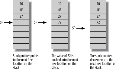
Stacks
Many processors implement one or more stacks , which serve as temporary storage in external memory. The processor can push a value from a register on the stack to preserve it for later use. The processor retrieves this value by popping from the stack back into a register. In some processor architectures, popping is also known as pulling.
Most processors have a special register known as a stack pointer , which references the next free location on the stack. Some processors implement more than one stack and so have more than one stack pointer. Most stacks grow down through memory. (Some processors have stacks that grow up as the stack is filled.) When the processor pushes or pops a value to or from the stack, the stack pointer automatically decrements or increments to point to the next free location.
Figure 2-3 shows the steps that occur when the content of a register (in this case, 72) is pushed onto the stack. These steps are normally performed by a single instruction (for example, PSHA). First, the value is copied from the register and stored to the location pointed to by the stack pointer. The stack pointer is then decremented. Again, these operations take place automatically by executing a single push instruction.
Most processors automatically save registers to the stack when events such as interrupts occur. However, the stack is also available to you as a programmer to temporarily store values. Some processors have two stacks, with one reserved for system use and the other available to the application programmer.
Stacks are particularly useful for the temporary storage of data. For example, let’s say we wish to call a subroutine, but we know that the subroutine changes the contents of the B accumulator as part of its operation. If there was nothing of importance in the B accumulator before we called the subroutine, this would be of little consequence. But if we wished to preserve the B accumulator, we would push the accumulator onto the stack before we called the subroutine and then pull it back after the subroutine ends:
PSHB       ; save B accumulator onto the stack
BSR   fred ; branch to subroutine fred
PULB       ; restore B accumulator from the stack
In this way, we have used the stack as a temporary storage location for data that we required later in the program. Alternatively, a good programmer would write the subroutine to preserve any affected registers:
fred
      PSHB  ; save B accumulator onto the stack
            ;
            ; (subroutine code here)
            ;
      PULB  ; restore B accumulator from the stack
      RTS   ;
Timing of Instructions
On some processors, particularly CISC chips, different instructions take varying lengths of time to complete. Sometimes it is important to know how long a given section of code will take to execute, particularly if the software is interacting with a time-critical external system. The execution time can be calculated by looking up the number of cycles each instruction takes and adding them together.
Tip
A “cycle” relates to the internal clock that is driving the processor. This is not necessarily the same speed as the crystal. The datasheet will tell you how the crystal frequency relates to the internal clock for a given processor.
The following example shows some 68HC11 assembly language and the number of cycles associated with each instruction:
      LDAA #$0F ; 2 cycles
again DECA      ; 2 cycles
      BNE again ; 3 cycles
exit  JMP $1000 ; 3 cycles
From examining the code, we can see that the loop is executed 15 (0x0F) times. This loop comprises five cycles in total. Therefore, the above program will take:
2 + (15 * 5) + 3 cycles = 80 cycles
For a 2 MHz 68HC11, a cycle is 500 ns. Hence, this code fragment will take 40,000 ns (or 40 μsecs) to complete.
Knowing the timing of instructions is often very useful. For example, suppose we need to have a program that will provide a delay of approximately 9 msec. To do this, we need to load a value into a register and count it down to zero. This will provide the delay.
So a program that would do this is simply:
       LDX #some_number ; load X with a number
repeat DECX             ; count down            3 cycles
       BNE repeat       ; not zero, repeat      3 cycles
For a 2 MHz 68HC11, a cycle is 500 ns. So for 9 msec, we require 18,000 cycles. The loop takes six cycles per iteration. Therefore, we need to run through the loop 3,000 times. In hex, 3,000 is 0x0BB8. So our program becomes:
       LDX #$0BB8   ; load X with 3000 decimal
repeat DECX         ; count down         3 cycles
       BNE repeat   ; not zero, repeat   3 cycles
Now, let me make some important points here. If an interrupt occurs during the loop, the processor will service the interrupt, and this will add an unknown (and unknowable) delay to the execution. If this code was controlling something critical, such an event would be disastrous. Most processors have instructions to disable and re-enable interrupts, and you would be well advised to turn off all interrupts prior to this code executing. Of course, you have to remember to re-enable them afterward as well. The other important point is that this code will provide a delay only of 9 msec, provided it is running on a 68HC11 at 2 MHz. If the code were run on a computer with a processor kicking along at 2.1 MHz, we would not get our 9 msec delay. In other words, techniques like this are not very portable and are generally considered bad practice. Use it only if you really have to. Programmers using code such as this often get caught when they move their code to a newer version of the hardware. Code that used to work is suddenly broken.
A better way to provide a fixed delay is to use a hardware timer, either as an internal peripheral to the microcontroller (and most have them) or as an external device. The timer generates an interrupt to the processor, and this gives a much more precise, reliable, and portable way of implementing a timing delay.