One of the fun things you can do with an embedded computer is getting it to actually move something, whether it be an external system or the embedded computer itself. Motion implies motor, and this section will look at how you interface an embedded computer to an electric motor. The possible applications could range from controlling locomotives on your model railroad layout to experiments in robotics and anything in between. A note of caution though: if your hardware and software are responsible for moving a physical object, then a bug can easily cause physical damage too. So, be careful.

Let’s say that we have an electric motor that operates from a 12V supply. Applying 12V across the motor will cause it to turn at full speed. Similarly, by applying 6V, we can get the motor spinning at half-speed. By varying the applied voltage, we can vary the speed at which the motor turns.

This voltage to drive the electric motor may be generated in several ways. The most obvious may seem to be to use a DAC to generate an analog output voltage and then use an amplifier to boost the signal to the voltage and current required to turn the motor. The speed of the motor is proportional to the output voltage. However, this technique has a major drawback. For very low-speed operation, the required output voltage may be too low to actually cause the motor to turn.

A better way is to use PWM. Consider the PWM signal in Figure 12-27, with an amplitude of 12V.

Figure 12-27. PWM signal with a 10% duty cycle

With a 10% duty cycle, the effective analog output voltage of this PWM signal is 1.2V. Now, by itself, 1.2V may not be enough to turn a motor. But, we’re not using 1.2V; we’re actually pulsing the motor with 12V, its maximum drive voltage. The duration of the pulses gives the equivalent speed of a motor voltage of 1.2V. However, by using a full 12V amplitude, we’re ensuring that the motor will turn. This is the advantage of PWM. To control speed, we vary the width of the pulse and not the amplitude.

Using PWM, you can get very slow motor speeds and very fine control. The pulses can cause a jerkiness to the motor if the overall frequency is low, but by choosing a high frequency, the jerkiness is averaged out.

Many microcontrollers, such as the PICs, the AVRs, and the DSP56805 we saw in Chapter 8, have internal, software-programmable PWM modules that make generating PWM signals easy. Even if a processor does not have a PWM module, you can still generate PWM under software control, simply by using a digital output line.

Let’s now take a look at how you would interface a processor to an electric motor using PWM. Due to the voltages and currents required by motors, you cannot simply hang a motor off the pins of a processor and expect it to work. You need an interface circuit that will take your logic-level, PWM output, and use this to switch much higher voltages and currents.

Figure 12-28 shows a conceptual model (in a crude and simplified form) of such an interface circuit, for driving a small electric motor. This type of circuit is known as an H-bridge.

Figure 12-28. Motor drive circuit using an H-bridge

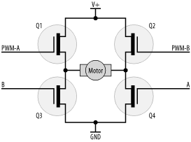
It’s not as confusing as it first looks. Don’t be too worried about the transistors in the circuit. They simply act as switches. Our motor operates from a supply voltage, V+. Apply V+ with one polarity and the motor turns in the forward direction. Reverse the polarity, and the motor reverses too. To drive the circuit, we use four outputs from the processor, two PWM (which I’ve called PWM-A and PWM-B), and two general I/O lines (which I’ve called A and B). Initially, all outputs are low, everything is turned off, and the motor is stationary.

If we send A high, the transistor Q4 turns on and connects the right “side” of the motor to ground. If we then send PWM-A high, the transistor Q1 turns on. Thus, the left “side” of the motor is connected to V+, and the motor spins. By generating a PWM signal on PWM-A, we can control the speed of the motor in that direction.

Conversely, by leaving A and PWM-A low and setting B and PWM-B high, transistor Q2 and transistor Q3 turn on, and the motor spins in the reverse direction. By generating a PWM signal on PWM-B, we can control the speed in the reverse direction.

Care must be taken in your software. If both Q1 and Q3 are turned on or both Q2 and Q4 are turned on, then you effectively connect V+ to ground, with very little resistance in between! The results would be spectacular and short-lived! A proper H-bridge circuit normally contains protection to prevent such a state from occurring.

The actual implementation of an H-bridge is a little more complicated and requires additional components such as protection diodes and so forth. Now, while you could design such an H-bridge circuit using discrete components, there is an easier way. A number of manufacturers, such as Motorola, International Rectifier (http://www.irf.com), M. S. Kennedy Corp (http://www.mskennedy.com), and others, make H-bridges in easy-to-use integrated circuits.

Let’s look at an example H-bridge, the Motorola MC33186. This chip is more sophisticated than the simple H-bridge I used to explain the concept. It provides more functionality yet is easier to control. This chip can operate from a supply voltage (V+) of between 5V and 28V and can switch continuous currents as high as 5A, yet it has logic inputs that are compatible with TTL levels. It has built-in short-circuit and overcurrent protection. Figure 12-29 shows an MC33186 circuit.

Figure 12-29. MC33186 motor drive circuit

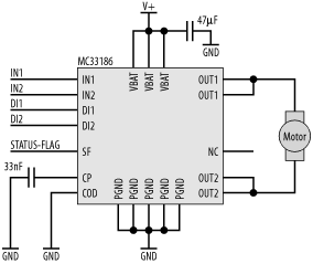
The chip has three power-supply inputs, V _BAT, all of which must be connected to the supply voltage, V+. The power-supply input needs to be decoupled using a 47μF capacitor. The internal charge pump also needs a decoupling capacitor. The pin, CP, provides access to the charge pump and requires a 33nF capacitor. The chip also has five ground pins, which, similarly, must all be connected to ground.

OUT1 and OUT2 are the pins that directly drive the motor. There are two of each, so that the high output currents are not traveling through a single pin.

IN1 and IN2 control both the motor’s speed and direction. DI1 and DI2 serve to disable the MC33186. These four control signals may be driven by a microcontroller’s I/O lines. For normal operation, DI1 is low and DI2 is high. Sending either DI1 high or DI2 low will disable the MC33186 and stop the motor. Table 12-1 shows how IN1, IN2, DI1, and DI2 affect the motor’s operation.

If we want the motor to run forward, we generate a PWM signal on IN1 and leave IN2 low. If we want to run the motor backward, we leave IN1 low and place a PWM signal on IN2. The duty cycle of the PWM signal determines the motor’s speed. Simple.

If IN1 and IN2 are in the same state, then there’s no voltage difference applied across the motor’s terminals, and so the motor is not driven.

Pin 2 of the MC33186, SF, is an output status flag. If the MC33186 is operating correctly, SF is high. If there is a fault, SF is driven low. SF may therefore be used as an interrupt to alert the host processor of a fault.

The input COD determines how the chip functions during a fault. If COD is left unconnected or is connected to ground, a change on either input DI1 or DI2 will reset the fault condition. If COD is connected to VCC (that’s +5V, not necessarily V+), then DI1 and DI2 are disabled. The fault condition can be reset only by a change on IN1 or IN2.

Using an integrated H-bridge circuit, such as the MC33186, greatly simplifies interfacing your embedded system to motors.

Sensing Motor Speed

The system that the motor is driving will affect the motor’s speed. If the motor must move a heavy load, then its actual speed of rotation may be less than the speed intended. In such situations, it is useful to measure the actual speed so that the embedded control system can compensate.

The easiest way to measure a motor’s rotational speed is to use an optical encoder module, such as the Agilent HEDS-9000 or a similar device. The encoder consists of a light source (LED) and an array of photodetectors, separated by a slotted disk known as a code wheel (Figure 12-30). The disk is mounted on the rotating motor shaft. Each time a slot passes between the LED and a detector, the detector receives a flash of light and generates an electrical pulse. The rate at which the pulses are generated corresponds directly to the rotational speed of the motor. The resolution of the code wheel is known as its counts per revolution, or CPR value. The HEDS series of encoders are available with CPRs ranging from 96 all the way up to 2048.

Figure 12-30. Block diagram of a HEDS-9000 optical encoder and a code wheel

The HEDS-9000 optical encoder operates from a 5V supply and has two outputs, A and B. These outputs are derived from two adjacent optical sensors. If the code wheel is rotating in one direction, output A will trigger before output B (Figure 12-31).

Figure 12-31. Output waveforms for the optical encoder

If the wheel is rotating in the opposite direction, then B will trigger before A (Figure 12-32).

Figure 12-32. Output waveforms for the optical encoder

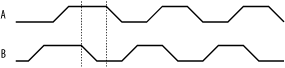
The rate at which the pulses arrive gives the motor’s speed, and the order in which they arrive shows the direction. This is known as quadrature encoding.

Most microcontrollers have timer/counter inputs that can measure external trigger events such as these. Under software control, you can use the timers to monitor these quadrature signals. However, Agilent makes a series of devices known as quadrature counters, the 12-bit HCTL-2000, the 16-bit HCTL-2016, and the 16-bit, cascadable HCTL-2020. These chips provide a bus-based interface to a processor and convert quadrature signals into a binary number representing motor position. A 16-bit position counter is capable of measuring 32,767 increments in either direction, which corresponds to approximately 15 turns of a 2048 CPR encoder. To determine the present motor speed or position, the processor simply reads from the quadrature counter as though it were just another memory location. Quadrature counters also have noise filters on their inputs and so provide a more reliable, and more accurate, way of determining motor position.

The schematics showing an optical encoder and quadrature counter are shown in Figure 12-33 and Figure 12-34. The optical encoder is placed on a separate, small PCB so that it may be easily mounted next to the motor’s shaft. The quadrature counter is located on the embedded computer’s PCB. IDC headers (J1 and J2) and a ribbon cable connect the two circuit boards.

Figure 12-33. Optical encoder circuit

Figure 12-34. Quadrature counter circuit

The quadrature counter requires a 14MHz clock. This is easily provided by an oscillator module. CHA and CHB are the quadrature inputs from the encoder. The counter has a reset input, RST, which clears the counter. Asserting RST zeros the quadrature counter and indicates that the motor is in the “home” position. This input is driven by a digital output of the microcontroller so that the counter can be reset under software control.

D0 to D7 are the data bus through which the processor reads the current position. Since the counters are either 12 bits or 16 bits, two reads are necessary to retrieve the value through the 8-bit bus. The counter therefore occupies two locations in memory, and the SEL input is used to select which byte is being read. If SEL is low, then the higher-order bits are read. If SEL is high, then the lower-order bits are read. To make these 2 bytes appear in adjacent memory locations, the processor’s address line, A0, is used to drive SEL. Thus, the least-significant address of the two selects the upper 8 bits, while the next address selects the lower 8 bits.

The counter does not have a chip select as such. Since it is a read-only device, the counter’s output enable, OE, functions as a combined chip select and output enable. Therefore, this input is driven by the output of the address decoder that corresponds to the region of the address space to which the counter is mapped. When the processor reads from that address range, OE is asserted, and the counter responds with data. Note that if the processor attempted to write to the counter, the counter would be selected and would respond with data. Therefore, both the processor and the counter would be attempting to drive data onto the data bus. This could potentially damage both chips. Now, with careful coding, this would not be a problem. However, a crashing program may inadvertently cause this situation to arise. To prevent this, a better solution is to include the processor’s read strobe as part of the address decode for this particular device. In other words, the counter is selected only if both the address is correct and the processor is performing a read. If the processor is performing a write to the counter’s address, the counter is not selected and the access is ignored.

A quadrature counter allows you to accurately monitor a motor’s position and speed.