2.2.1Characteristics of AL

1. Auto-knowledge

An autonomic learner can only be highly autonomous if he or she is at a high level of auto-awareness. Therefore, auto-knowledge is the basis for AL. The learner must have “auto-knowledge” to determine whether the current behaviour is compatible with the learning environment. New conditions and a new environment will give rise to new behaviour; therefore, auto-knowledge should be constantly updated and evolve according to the environment. In other words, auto-knowledge is the internal knowledge base of the AL system [9]. With such auto-knowledge, the learner’s self-learning ability will become stronger.

2. Auto-monitoring

Self-directed learning is a feedback cycle. AL individuals can monitor the effectiveness of their learning methods or strategies and adjust their learning activities based on this feedback. In the process of learning, auto-monitoring refers to the process of self-learning individuals assessing their learning progress using certain criteria. Auto-monitoring is a key process of AL. Self-directed learning is only possible when learners are self-monitoring [8]. Planning can be used to monitor the problem-solving process. Auto-monitoring strengthens the learner’s self-learning ability.

3. Auto-evaluating

The auto-evaluating process is the most important component of AL because it influences not only the ability judgment, task evaluation, goal setting, and expectation of learners but also the individual auto-monitoring of the learning process and the learning result of the self-strengthening [8].

Existing research suggests that auto-evaluating includes self-summary, self-assessment, self-attribution, self-strengthening, and other sub-processes. Self-assessment involves comparing the learning results with the established learning objectives, to confirm which goals have been completed, which goals have not yet been achieved, and then to judge the merits of self-learning. Self-attribution refers to a self-assessment based on the results of learning success or failure, reflecting the reasons for the follow-up learning providing experience or lessons. Self-reinforcement is the process of rewarding or stimulating oneself based on the results of self-assessment and self-attribution, and it often motivates subsequent learning [5].

Behavioural evaluation is a way of simulating the behaviour of AL individuals. When solving a problem, two simple evaluation methods can be selected: the first is to choose the best behaviour to perform, that is, in the current state, that which acts most toward the direction of the best move; the second is to choose a better behaviour, that is, choose an act that offers the superior direction.

When learning an action, the learner autonomously evaluates his or her behaviour using the current evaluation function. The evaluation function is described as follows.

The original objective function value of the learner’s self-learning is that a new situation is obtained after the execution of an action. The corresponding new objective function is denoted by [1, 2, ..., n], where n is the number of objective functions.

The historical evaluation function is adjusted as follows:

where VYi denotes the historical evaluation function, VYi denotes the new evaluation function, and α denotes the weighting coefficient.

Auto-evaluation enhances the AL ability of the learner.

2.2.2Axiom system of AL subspace [7]

The various problems in the real world can be described by learning space. That is mapping learning problems into learning space. A learning problem can be mapped into multiple learning spaces, and a learning space can be used to describe multiple learning problems [4].

Definition 2.1 Learning space: The space used to describe the learning process is called the learning space. It consists of five parts: {learning sample, learning algorithm, input data, output data, representation theory}, which can be expressed as S = {EX, ER, X, Y, ET}.

Definition 2.2 Learning subspace: A spatial description of a specific learning problem, that is, a subset of the learning space, is called the learning subspace.

The axiom system of the AL subspace consists of two parts: (1) a set of initial formulas, namely axioms, and (2) a number of deformation rules, namely deduction rules.

First, on the basis of DFL, we define AL as follows:

Definition 2.3 Autonomic learning: $\left(\overleftarrow{AL},\overrightarrow{AL}\right)$ refers to the mapping of an input dataset $\left(\overleftarrow{X},\overleftarrow{X}\right)$ to an output dataset $\left(\overleftarrow{Y},\overleftarrow{Y}\right)$ in an AL space, which can be expressed as $\left(\overleftarrow{AL},\overrightarrow{AL}\right):\left(\overleftarrow{X},\overrightarrow{X}\right)\to \left(\overleftarrow{Y},\overrightarrow{Y}\right).$ According to $\left(\overleftarrow{AL},\overrightarrow{AL}\right),$ the process can be divided into 1:1 AL, n:1 AL, 1: n AL, and m: n AL.

AL can be divided into the following modes according to the knowledge stored in the knowledge base (KB): When the KB is the empty set, there is no a priori knowledge, only 1:1 or n:1 AL. As the learning process continues, the KB grows and updates itself, enabling 1: n or m: n AL.

Definition 2.4 Autonomic learning space: The space used to describe the learning process is composed of all AL elements, called the AL Space. It consists of five elements, which can be expressed as $\left(\stackrel{\leftharpoonup }{S},\stackrel{\rightharpoonup }{S}\right)=\left\{\left(\overleftarrow{Ex},\overrightarrow{Ex}\right),ER,\left(\overleftarrow{X},\overrightarrow{X}\right),\left(\overleftarrow{Y},\overrightarrow{Y}\right),ET\right\},$ where $\left(\overleftarrow{S},\overrightarrow{S}\right)$ represents the AL space, $\left(\overleftarrow{Ex},\overrightarrow{Ex}\right)$ denotes the AL samples, ER is an AL algorithm, $\left(\overleftarrow{X},\overrightarrow{X}\right)\text{and}\left(\overleftarrow{Y},\overrightarrow{Y}\right)$ are the input and output data, respectively, and ET is the learning theory.

Definition 2.5 Autonomic learning subspace (ALSS): According to some standard, we divide the AL space $\left(\overleftarrow{S},\overrightarrow{S}\right)$ into n subspaces: $\left({\overleftarrow{S}}_1,{\overrightarrow{S}}_1\right),\left({\overleftarrow{S}}_2,{\overrightarrow{S}}_2\right),\dots ,\left({\overleftarrow{S}}_i,{\overrightarrow{S}}_i\right),\dots ,$$\left({\overleftarrow{S}}_n,{\overrightarrow{S}}_n\right),\text{that is},\left(\overleftarrow{S},\overrightarrow{S}\right)=\left({\overleftarrow{S}}_1,{\overrightarrow{S}}_1\right),\left({\overleftarrow{S}}_2,{\overrightarrow{S}}_2\right),\dots ,\left({\overleftarrow{S}}_i,{\overrightarrow{S}}_i\right),\dots ,\left({\overleftarrow{S}}_n,{\overrightarrow{S}}_n\right),i=1,2,\dots ,n.$

ALSS is a learning subspace with the highest and lowest limits, namely, $S_{\min },S_{\max }ϵR^n\left(\overleftarrow{S_{\min }},\overrightarrow{S_{\min }}\right)\le \left({\overleftarrow{S}}_i,{\overrightarrow{S}}_i\right)\le \left(\overleftarrow{S_{\max }},\overrightarrow{S_{\max }}\right)\}.$ In the algorithm, it can be regarded as the subspace of algorithm optimization. In this subspace, some AL individuals are distributed, and the corresponding search ability of the individuals is given, so that they can carry out AL in the corresponding environment.

The relationship between the AL space and ALSS is depicted graphically in Fig. 2.1.

The partition given in Definition 2.5 is complete, and the axioms can be derived as follows:

Axiom 2.1 $\left(\overleftarrow{S},\overrightarrow{S}\right)={\displaystyle \underset{i=1,n}{\cup }\left({\overleftarrow{S}}_i,{\overrightarrow{S}}_i\right).}$

Axiom 2.2 $\forall \left({\overleftarrow{S}}_i,{\overrightarrow{S}}_i\right)ϵ\left(\overleftarrow{S},\overrightarrow{S}\right),i=1,2,\dots ,n,\left({\overleftarrow{S}}_i,{\overrightarrow{S}}_i\right)\subseteq \left({\overleftarrow{S}}_i,{\overrightarrow{S}}_i\right).$

Axiom 2.3 If $\left({\overleftarrow{S}}_i,{\overrightarrow{S}}_i\right)\subseteq \left({\overleftarrow{S}}_j,{\overrightarrow{S}}_j\right),\left({\overleftarrow{S}}_j,{\overrightarrow{S}}_j\right)\subseteq \left({\overleftarrow{S}}_i,{\overrightarrow{S}}_i\right),i,j=1,2,\dots ,n.\text{then}\left({\overleftarrow{S}}_i,{\overrightarrow{S}}_i\right)=$$\left({\overleftarrow{S}}_i,{\overrightarrow{S}}_i\right).$

Axiom 2.4 If $\left({\overleftarrow{S}}_i,{\overrightarrow{S}}_i\right)\subseteq \left({\overleftarrow{S}}_j,{\overrightarrow{S}}_j\right),\left({\overleftarrow{S}}_j,{\overrightarrow{S}}_j\right)\subseteq \left({\overleftarrow{S}}_k,{\overrightarrow{S}}_k\right),i,j,k=1,2,\dots n,\text{then}\left({\overleftarrow{S}}_i,S_i\right)$$\left({\overleftarrow{S}}_k,{\overrightarrow{S}}_k\right).$

2.3.1Preparation of algorithm

AL individuals in the ALSS can be seen as vectors.

1. Definition of variables

The state of an AL individual can be expressed by the vector $\left(\overleftarrow{X},\overrightarrow{X}\right)=$$\left\{\left({\overleftarrow{x}}_1,{\stackrel{\leftharpoonup }{x}}_1\right),\left({\overleftarrow{x}}_2,{\stackrel{\leftharpoonup }{x}}_2\right),\dots ,\left({\overleftarrow{x}}_n,{\stackrel{\leftharpoonup }{x}}_n\right)\right\},$ where $\left({\overleftarrow{x}}_i,{\overrightarrow{x}}_i\right)\left(i=1,2,\dots ,n\right)$ is the variable to be optimized; the objective function value $Y=f\left(\left(\stackrel{\leftharpoonup }{X},\stackrel{\rightharpoonup }{X}\right)\right)$ represents the learner’s current object of interest, Learner_consistence; $d_{ij}=\left|\right|\left({\overleftarrow{X}}_i,{\overrightarrow{X}}_i\right)-\left({\overleftarrow{X}}_i,{\overrightarrow{X}}_i\right)\left|\right|$ represents the distance between AL individuals; Visual represents the perceived distance of AL individuals; Step represents the maximum number of steps moved by AL individuals; and δ represents the congestion degree of AL individuals.

The neighbourhood of AL organization is defined as follows:

2. Description of behaviour

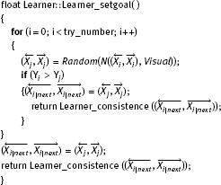
(1)Setting target behaviour

Let the current state of AL individual Learner be $\left({\overleftarrow{X}}_i,{\overrightarrow{X}}_i\right),$ and choose a state $\left({\overleftarrow{X}}_j,{\overrightarrow{X}}_j\right)$ at random in the corresponding sensing range. If Yi is less than Yj, go forward a step in that direction; otherwise, choose another state $\left({\overleftarrow{X}}_j,{\overrightarrow{X}}_j\right)$ at random to judge whether or not the forward condition is satisfied. If the forward conditions are not met after a specified number of attempts, then perform some other behaviour (such as moving a step at random).

The pseudocode description of this process is shown in Algorithm 2.1, where Random$\left(N(({\overleftarrow{X}}_i,{\overrightarrow{X}}_i\right),$ Visual)) represents a randomly selected neighbour in the neighbourhood of the visual distance of $\left({\overleftarrow{X}}_j,{\overrightarrow{X}}_j\right)$

(2)Aggregation behaviour

let $\left({\overleftarrow{X}}_j,{\overrightarrow{X}}_j\right)$ be the current state of AL individual Learner, and let n be the number of learning partners while exploring the current neighbourhood (which is dij < Visible). If nm / N (0 < 1), the learning partner centre has more learning objects but is not crowded. Under the condition Yi < Yc, move a step toward the centre of the learning partner; otherwise, perform other behaviours (such as setting the target behaviour).

The pseudocode description of this process is shown in Algorithm 2.2:

(3)Imitating behaviour

Let $\left({\overleftarrow{X}}_j,{\overrightarrow{X}}_j\right)$ be the current state of AL individual Learner, and explore the neighbour $\left(\overleftarrow{X_{\max }},\overrightarrow{X_{\max }}\right)$ with the best state in the current neighbourhood.

Let n be the number of learning partners of the neighbour $\left(\overleftarrow{X_{\max }},\overrightarrow{X_{\max }}\right)$ If $Y_i<Y_{\max }\text{with}\frac{n_m}{N}<\delta \left(0<\delta <1\right),$ then there is high Learner_consistence near the learning partner $\left(\overleftarrow{X_{\max }},\overrightarrow{X_{\max }}\right)$ without being crowded. Thus, the Learner moves a step toward the learning partner $\left(\overleftarrow{X_{\max }},\overrightarrow{X_{\max }}\right);$ otherwise, some target setting behaviour is performed.

The pseudocode description of this process is shown in Algorithm 2.3.

(4)Random behaviour

The realization of random behaviour is relatively simple. A state in a smaller neighbourhood is selected at random, and Learner moves in that direction. This ensures that the AL object will not be far away from the better ALSS in the blind moving process. Other autonomic learners who did not find the learning goal would conduct stochastic learning behaviour in their neighbourhood D.

In fact, the random learning behaviour is the default target setting behaviour.

(5)Auto-evaluating behaviour

After learning an action, the learner autonomously evaluates his or her behaviour using the current evaluation function. The evaluation function is described as follows.

Let Yi be the original objective function value of Learner, and consider a new situation obtained after performing an action. The corresponding new objective function value is ${Y^{\prime }}_t,\text{denoted as}{D}_i=Y_i-{Y^{\prime }}_i,\text{where}i\in \left[1,2,\dots ,n\right]$ and n denotes the number of objective functions.

The historical evaluation function is adjusted as follows:

where VYi denotes the historical evaluation function, VYi denotes the new evaluation function, and denotes the weighting coefficient.

This auto-evaluation process strengthens the AL ability of Learner. The pseudocode description of this process is shown in Algorithm 2.4.

2.3.2Algorithm of ALSS based on DFL

In the process of learning, the changing environment and lack of complete information make it difficult to predict the exact model of the environment. Traditional supervised learning methods cannot perform behaviour learning in an unknown environment, so Learner must exhibit intelligent behaviour. Intensive learning, as an atypical learning method, provides agents with the ability to select the optimal action in the Markov environment, and obviates the need to establish the environment model. This approach has been widely used in the field of machine learning with a certain degree of success. However, intensive learning has some limitations: (1) single-step learning is inefficient and can only accept discrete state inputs and produce discrete actions, but the environment in which machine learning is usually spatially continuous. (2) Discretization of continuous state space and motion space often leads to information loss and dimension disaster. (3) The computational complexity increases exponentially with the increase of the state-action pairs. Trial-and-error interactions with the environment can bring about losses in the system.

In view of the above limitations of reinforcement learning, this section proposes an AL mechanism based on DFL. According to the learner’s AL performance, the learning mechanism is decomposed into multi-step local learning processes. The state space is divided into a finite number of categories, which reduces the number of state-action pairs. After receiving an input state vector, the learner chooses an action to execute through a dynamic fuzzy reasoning system, and continuously updates the weight of the result in the rule base until convergence. Thus, a complete rule base can be obtained, which provides prior information for the learner’s behaviour.

1. Reasoning model of DF

The reasoning process of DFL attempts to solve the problem of dynamic fuzziness. The model can be expressed as:

where DF(A), DF(A1), DF(A2), ..., DF(An) are the prerequisites or conditions of dynamic fuzzy reasoning, DF(C) is the conclusion or posterior of dynamic fuzzy reasoning, and DF(R) is the dynamic fuzzy relation between the premise and the conclusion satisfied by DF(R) ∈ [0, 1] × [←,→]. The premises and conclusions are facts represented by DFL.

The rule base for a dynamic fuzzy inference system is generally composed of n rules in the following form:

where Rj represents the j th rule.

2. Description of algorithm

The goal of Q-learning is to learn how to choose the suboptimal or optimal action according to the external evaluation signal in the dynamic environment. The essence is of a learning process of dynamic decisions. However, the relevant environmental information may be lost when the learner does not have complete knowledge of the environment. Thus, a trial-and-error method must be used, and so the efficiency of the algorithm is not high. Sometimes, learning in an unknown environment can also involve some risks. One way to reduce these risks is to use an environmental model. The environmental model can be built using the experience gained by performing the relevant tasks before. Using environmental models can facilitate the results of the action without risking losses.

The environment model is a function from the state and action (St+1, a) to the next state and the enhanced value (St+1, r). The model is established in the following two ways: first, the agent builds the model offline using the data provided in the initial stage of the learning; second, the agent establishes or perfects the environment model online in the process of interacting with the environment. We consider the second method in AL.

In this chapter, we add the function E: S × A → R, which represents the knowledge of experience. This function influences the learner’s choice of action in the process of AL, thus accelerating the convergence speed and learning speed of the algorithm.

Definition 2.6 Experience: Experience is represented by a four-tuple $\{\left({\overleftarrow{S}}_t,{\overrightarrow{S}}_t\right),a_t,$$\left(\overleftarrow{S_{t+1}},\overrightarrow{S_{t+1}}\right),r_t\}$ indicating that an action at is performed at state $\left({\overleftarrow{S}}_t,{\overrightarrow{S}}_t\right)$ generating a new state $\left(\overleftarrow{S_{t+1}},\overrightarrow{S_{t+1}}\right)$ and obtaining an enhanced signal rt at the same time.

The empirical function $E\left(\left(\overleftarrow{S},\overrightarrow{S}\right),a\right)$ in the AL algorithm records the relevant empirical information about performing a in state $\left(\overleftarrow{S},\overrightarrow{S}\right).$ The most important problem when adding an empirical function to an algorithm is how to obtain empirical knowledge in the initial stage of learning, that is, how to define the empirical function $E\left(\left(\overleftarrow{S},\overrightarrow{S}\right),a\right).$ The answer mainly depends on the specific field to which the algorithm is applied. For example, in the case of agent-based routing optimization, when the agent collides with the wall, the corresponding knowledge is acquired. That is, the agent obtains empirical knowledge about the environmental model online in the process of interacting with the environment.

We assume that the rule base described in the previous section has been established. This rule base can be used by the AL individual to select an action. According to the output value and empirical function of the dynamic fuzzy reasoning system for action selection, the environment goes into the next state and returns a certain value. According to the return value of this action, the result weights are updated in the KB.

The pseudocode of the autonomic subspace learning algorithm based on DFL is shown in Algorithm 2.5.

The demand for initial values in the algorithm is not high: usually, initializing a random distribution of Learners in the variable domain using ::Learner_init(); the algorithm can be terminated according to the actual situation, such as whether the variance between the values of successive results is less than the expected error.

The characteristics of our autonomic subspace learning algorithm based on DFL can be summarized as follows:

(1)The autonomic subspace learning algorithm based on DFL takes the learning objective as the objective function of the algorithm in the learning process (equivalent to the optimization process). The algorithm only compares the objective function values and does not consider other specific problems of the traditional optimization algorithm (such as derivative information). The nature of the objective function is not computationally complex. Therefore, the ALSS algorithm based on DFL can be considered a type of “black box” algorithm.

(2)Without high demands on the initial value, the algorithm only needs to initialize a number of AL individuals at random in the learning subspace to generate the initial value of the algorithm.

(3)In the process of optimization, there are relatively few parameter settings, mainly related to giving the behaviour process of the individuals a larger allowable range.

(4)The autonomic subspace learning algorithm based on DFL is very robust, which means that the algorithm gives similar results to the same problem under different run conditions.

2.3.3Case analysis

1. Experiment description

Using Java as a development tool, the autonomic subspace learning algorithm was applied in a 10 × 10 grid environment. The experimental environment is shown in Fig. 2.2. Each square represents a state of the Learner. Box 2 is the Learner’s initial position, Box 3 represents the Learner’s target position, and Region 1 is the obstacle. The obstacles and targets in the environment are static. For the Learner, the environment (obstacles, boundaries, and the location of the target) is unknown. In the Learner-centred two-dimensional space, the four directions of motion are equally distributed. The Learner’s four directions of movement, East, West, South, and North, represent four optional actions. If the Learner encounters obstacles or boundaries, then he must return to the original state.

The parameters of the standard Q-learning algorithm and autonomic subspace learning algorithm based on DFL were set to a = 0.1, r{100, 100, 0}, and the corresponding condition was {hit obstacles, reach the target, other}.

2. Experiment results

Using the autonomic subspace learning algorithm based on DFL (denoted as Method I) and Q-learning algorithm (denoted Method II), we compared the time cost and average number of search steps (L) required for the Learner to reach the target. The experimental results are shown in Figs. 2.3 and 2.4. The Episodes in Reinforcement Learning denote the learning cycle, i.e. the process in which the Learner moves from the initial position to the target position. Steps represents the number of steps taken by the Learner in moving from the initial position to the target position in each learning cycle.

In Fig. 2.3, it can be seen that, with the increase in the number of experiments, the autonomic subspace learning algorithm based on DFL required much less time than the Q-learning method.

Figure 2.4 shows that, with the increase in the number of experiments, the average number of search steps in method I is much smaller than that in method II.

In summary, the experiment shows that, in the 10 × 10 grid, the autonomic subspace learning algorithm based on DFL achieves a faster learning rate and better convergence ability than the ordinary Q-learning method.

References

[1]Pang WG. Self-regulated learning. Shanghai, China, East China Normal University Edition, 2003.
[2]Shen WM. Discovery as autonomous learning from the environment. Machine Learning, 1993, 12(8): 143–165.
[3]Wang GY, He X. Initiative machine learning based on rough set. Computer Science, 2002, 29(9): 24–26.
[4]Chen F, Li FZ. A Preliminary study on the theory and algorithm of learning subspace orbital generation for lie group machine learning. Journal of Soochow University (Nature Science Edition), 2007, 23(1): 61–66.
[5]Wang J. Research and application on learning algorithm of autonomic learning subspace based on DFL. Master’s thesis, Soochow University, Suzhou, China, 2008.
[6]Wang J, Li FZ. Axiomatic system of autonomic learning subspace based on DFL. Computer Science, 2008, 35(12): 146–148.
[7]Wang J, Li FZ. Autonomic learning model and algorithm based on DFL. In Proceedings of 2007 IEEE International Conference on Granular Computing, Silicon Valley, USA, 2007, 259–265.
[8]Cofino T, Doganata Y, Drissi Y, et al. Towards knowledge management in autonomic systems. In Proceedings of the Eighth IEEE International Symposium on Computers and Communication, 2003, 2: 789–794.
[9]Li FZ. Dynamic fuzzy logic and its applications. New York, USA, Nova Science Publishers, 2008.