
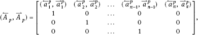
(1.8) can be rewritten as
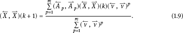
Since the right side of (1.9) is equal to the origin in the domain is the equilibrium point of (1.9).
Theorem 1.3 The equilibrium point of (1.9) of the DFMLS is globally asymptotically stable. If there exists a positive dynamic fuzzy matrix then [18]
Proof: Consider the following Lyapunov function:
![]()
where is a positive dynamic fuzzy matrix. Then, there is


is obtained from (1.10) and Using the Lyapunov stability theorem, the proof is complete.
1.2.3DFML geometric model description
1.2.3.1Geometric model of DFMLS [8, 11]
As shown in Fig. 1.3, we define the universe as a dynamic fuzzy sphere (large sphere), in which some small spheres represent the DFSs in the universe. Each dynamic fuzzy number is defined as a point in the DFS (small sphere). The membership degree of each dynamic fuzzy number is determined by the position and radius of the DFS (small sphere) in the domain (large sphere) and the position in the DFS (small sphere).
1.2.3.2Geometric model of DFML algorithm
In Fig. 1.4, the centre of the two balls is the expected value the radius of the large sphere is and the radius of the sphere is and are the same as in Algorithm 1.2].
The geometry model can be described as follows:
(1)If the value of the learning algorithm falls outside the ball, then this learning is invalid. Discard and feed the information back to the rules of the system library and learning part, then begin the process again;
(2)If the value of the learning algorithm falls between the big sphere and the small sphere, the information is fed back to the system rules and learning part of the library so that they can be amended. Proceed to the next step;
(3)If the value of the learning algorithm falls within the small sphere, it is considered that the precision requirement has been reached. Terminate the learning process and output

1.2.4Simulation examples
Example 1.1 The sunspot problem: Data from 1749–1924 were extracted from [19]. This gave a total of 176 data, of which the first 100 were used as training samples and the remainder were used as test data.
Figure 1.5 shows the error and iterative steps of the algorithm described in this section, the neural network elastic Back Propagation (BP) algorithm resilient propagation (RPROP) [20], and a Q-learning algorithm. When the error RPROP falls into a local minimum and requires approximately 1660 iterations to find the optimum solution; in the Q-learning algorithm, 1080 iterations are needed to reach an error of for our algorithm, the number of iterations required for an error of is 455. When the error the training is basically stable, and the required number of iterations is about 1050. Figure 1.6 compares the actual values with the predicted values obtained by the algorithm presented in this section for an initial value ) gain learning coefficient of α = 0.3, correction coefficient of β = 0.2, maximum tolerance error of acceptable error of and error
Example 1.2 Time series forecast of daily closing price of a company over a period of time.
The data used in this example are again from [19]. Of the 250 data used, the first 150 data were taken as training samples, and the remaining 100 were used as test data.


We set the initial value to gain learning coefficient to α = 0.3, correction coefficient to β = 0.3, maximum tolerance error to and acceptable error to
Figure 1.7 shows the error and iterative steps of this algorithm compared with the elastic BP algorithm RPROP and the BALSA algorithm, which is based on a Bayesian algorithm [21]. When the performance index is RPROP falls into a local minimum after approximately 146 iterations; for the BALSA algorithm, when the performance index is the number of iterations required is 114; for our algorithm, when the performance index is less than the number of iterations required is 82. The number of iterations required to satisfy the accuracy requirement is about 500. Figure 1.8 compares the actual values and the learning results of the proposed algorithm, where k is the number of iterations.
1.3Relative algorithm of DFMLS [5]
1.3.1Parameter learning algorithm for DFMLS
1.3.1.1Problem statement
According to Algorithm 1.2, DFMLS adjusts and modifies the rules in the rule base according to the results of each learning process. The adjustment and modification of rules are mainly reflected in the adjustment of parameters in the rules. For this problem, this section derives a DFML algorithm that identifies the optimal system parameters.

Consider the DFMLS described in the previous section, which is formalized as is
![]()
where are the mean and variance of the corresponding membership functions.
According to the given input and output data pairs 1, 2, . . ., N), the system parameters can be learnt using the least-squares error (LSE) objective function, which minimizes the output error of the system:
and modifies the parameters along the direction of steepest gradient descent:
where η is the training step length. Thus, the iterative optimization equation of parameter can be obtained so as to minimize the sum of squares of the error in (1.11).
There are two issues worth considering:
(1)The choice of step size: If only a single fixed training step is used, it is difficult to take into account the convergence of different error variations, sometimes resulting in oscillations in the learning of the parameters, especially near the minimum point. Fixed training steps will reduce the convergence speed. In practical applications, there is often no universal, fixed training step for different parameter learning problems. Therefore, the following optimization steps are proposed to solve this problem [22]: