(2)When the input and output data contain measurement noise, the learning parameter cannot converge to the true value ${\left(\overleftarrow{\theta },\overrightarrow{\theta }\right)}^{*}$ using the LSE objective function.

When the input and output data contain noise, the input and output data pairs can be expressed as:

where ${\left({\overleftarrow{X}}_k,{\overleftarrow{X}}_k\right)}^{*},{\left({\overleftarrow{Y}}_k,{\overrightarrow{Y}}_k\right)}^{*}$ are the true values of the input and output data, respectively, $n_{\left({\overleftarrow{X}}_k,{\overrightarrow{X}}_k\right)},n_{\left({\overleftarrow{Y}}_k,{\overleftarrow{Y}}_k\right)}$ are the input and output data contained in the noise, respectively, and the variance is $\left\{{\left(\overleftarrow{\delta },\overrightarrow{\delta }\right)}_{\left({\overleftarrow{x}}_k^1,{\overleftarrow{x}}_k^1\right)},i=1,2,\mathrm{...},n\right\},{\left(\overleftarrow{\delta },\overrightarrow{\delta }\right)}_{\left({\overleftarrow{y}}_k,{\overleftarrow{y}}_k\right)}.$

When learning the parameter of a DFMLS that includes input/output noise, the error cost function [30] is defined as

$\begin{array}{rl}& E_{EIV}=\frac{1}{2}\sum _{k=1}^N\left[\frac{{\left(\left({\stackrel{\leftharpoonup }{y}}_k,{\stackrel{\rightharpoonup }{y}}_k\right)-<!--\; -\; -->f((\stackrel{\leftharpoonup }{\theta },\stackrel{\rightharpoonup }{\theta }),({\stackrel{\leftharpoonup }{X}}_k,{\stackrel{\rightharpoonup }{X}}_k{)}^{\prime }\right)}^2}{{\left(\stackrel{\leftharpoonup }{\mathrm{\delta <!--\; d\; -->}},\stackrel{\rightharpoonup }{\mathrm{\delta <!--\; d\; -->}}\right)}_{\left({\stackrel{\leftharpoonup }{y}}_k,{\stackrel{\rightharpoonup }{y}}_k\right)}^2}+\sum _{i=1}^n\frac{{(({\stackrel{\leftharpoonup }{x}}_k^i,{\stackrel{\rightharpoonup }{x}}_k^i)-<!--\; -\; -->({\stackrel{\leftharpoonup }{x}}_k^i,{\stackrel{\rightharpoonup }{x}}_k^i{)}^{\prime })}^2}{{\left(\stackrel{\leftharpoonup }{\mathrm{\delta <!--\; d\; -->}},\stackrel{\rightharpoonup }{\mathrm{\delta <!--\; d\; -->}}\right)}_{\left({\stackrel{\leftharpoonup }{x}}_k^i,{\stackrel{\rightharpoonup }{x}}_k^i\right)}^2}\right],\\ & =\frac{1}{2}\sum _{k=1}^N\left(\frac{{\left(\stackrel{\leftharpoonup }{e},\stackrel{\rightharpoonup }{e}\right)}_{({\stackrel{\leftharpoonup }{y}}_k,{\stackrel{\leftharpoonup }{y}}_k)}^2}{{\left(\stackrel{\leftharpoonup }{\mathrm{\delta <!--\; d\; -->}},\stackrel{\rightharpoonup }{\mathrm{\delta <!--\; d\; -->}}\right)}_{({\stackrel{\leftharpoonup }{y}}_k,{\stackrel{\leftharpoonup }{y}}_k)}^2}+\sum _{i=1}^n\frac{{\left(\stackrel{\leftharpoonup }{e},\stackrel{\rightharpoonup }{e}\right)}_{\left({\stackrel{\leftharpoonup }{x}}_k^i,{\stackrel{\rightharpoonup }{x}}_k^i\right)}^2}{{\left(\stackrel{\leftharpoonup }{\mathrm{\delta <!--\; d\; -->}},\stackrel{\leftharpoonup }{\mathrm{\delta <!--\; d\; -->}}\right)}_{\left({\stackrel{\leftharpoonup }{x}}_k^i,{\stackrel{\rightharpoonup }{x}}_k^i\right)}^2}\right)\left(1.14\right)\end{array}$

where ${\left({\overleftarrow{X}}_k,{\overleftarrow{X}}_k\right)}^{\text{'}}$ is the estimate of the true value ${\left({\overleftarrow{X}}_k,{\overleftarrow{X}}_k\right)}^{*}.$

Theorem 1.4 When the input and output data contain noise, the learning parameter $\left(\overleftarrow{\theta },\overrightarrow{\theta }\right)$ converges strongly to the true value ${\left(\overleftarrow{\theta },\overrightarrow{\theta }\right)}^{*}$ of the parameters using the error cost function of (1.14), which is

Proof: The proof is easy using the proof of Lemma 2 in [23].

1.3.1.3Examples

To verify the validity of the parameter-learning algorithm for the DFMLS proposed in this section, and to illustrate the superiority of this algorithm, we simulate the nonlinear function proposed in [22]. Finally, the algorithm is compared with the algorithm in [22]:

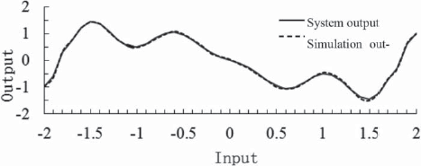
where $\left(\overleftarrow{x},\overrightarrow{x}\right)\in \left[\left(-\overleftarrow{2},-\overrightarrow{2}\right),\left(-\overleftarrow{2},-\overrightarrow{2}\right)\right],\mathrm{and}{\left(\overleftarrow{v},\overrightarrow{v}\right)}_x$ is random interference noise with mean $\left(\overleftarrow{0},\overrightarrow{0}\right)$ and mean square error $\left(0.03\overleftarrow{2},0.03\overrightarrow{2}\right).$

A total of 200 input and output points $\left(\left({\overleftarrow{X}}_k,{\overleftarrow{X}}_k\right)\left({\overleftarrow{Y}}_k,{\overleftarrow{Y}}_k\right)\right)$ were uniformly selected as training samples. The noise variance of the input and output samples was set to ${\left(\overleftarrow{\delta },\overrightarrow{\delta }\right)}^2=\left(0.2\overrightarrow{5},0.2\overleftarrow{5}\right),$ and the subtraction clustering algorithm [24] was used to cluster the sample data. Thirty-two dynamic fuzzy logic (DFL) rules were extracted, and the corresponding initial parameters were determined. Using the adaptive parameter-learning algorithm proposed in [22] and the method proposed in this section, the algorithm trained 100 steps for the relevant parameters, where ${\eta }_{{\left(\overleftarrow{m},\overrightarrow{m}\right)}_{\left({\overleftarrow{A}}_1^l,{\overleftarrow{A}}_1^l\right)}}\left(0\right),{\eta }_{{\left(\overleftarrow{m},\overrightarrow{m}\right)}_{\left({\overleftarrow{A}}_1^l,{\overleftarrow{A}}_1^l\right)}}\left(0\right),{\eta }_{{\left(\overrightarrow{\delta },\overleftarrow{\delta }\right)}_{\left({\overleftarrow{b}}_i,{\overrightarrow{b}}_i\right)}}\left(0\right)$ was set to 0.01. The results are shown in Figs. 1.9 and 1.10. Figure 1.9 shows the simulated output of the adaptive parameter-learning algorithm, which has a root mean square error of RMSE = $\left(0.0560\overleftarrow{9},0.0560\overleftarrow{9}\right);$ Fig. 1.10 shows the parametric-learning algorithm described in this section, which has a root mean square error of RMSE = $\left(0.0417\overleftarrow{3},0.0417\overleftarrow{3}\right),$ Obviously, our algorithm is superior.

1.3.2Maximum likelihood estimation algorithm in DFMLS

Incomplete observations and unpredictable data losses in the process of learning mean that many real systems have a lot of missing data. Thus, studies on incomplete data have very important theoretical and practical value in terms of how to use the observed data to estimate the missing data in a certain range. Earlier solutions include the Expectation-Maximization (EM) algorithm [25] proposed by Dempster, Laird, and Rubin in 1977; the Gibbs sampling proposed by S. Geman and D. Geman in 1984; and the Metropolis-Hastings method proposed by Metropolis in 1953 and improved by Hastings. The EM algorithm has been extended into a series of algorithms, such as the EM algorithm proposed by Meng and Rubbin in 1993 and the Monte Carlo EM algorithm. The EM algorithm is an iterative procedure based on the maximum likelihood estimation (MLE) and is a powerful tool. The advantage of the EM algorithm is obvious, as it simplifies a problem through division, but its shortcomings cannot be ignored: its convergence rate is slow, and local convergence and pseudo-convergence phenomena [26] may also occur. The GEM algorithm and Monte Carlo EM algorithm offer various improvements, but the slow convergence rate has not been adequately dealt with. The α-EM algorithm for calculating the entropy rate in information theory can overcome this defect. Therefore, this paper proposes a dynamic fuzzy α-EM algorithm (DFα-EM) for the statistical inference problem of incomplete DFD in a DFMLS.