
The operator “ ≤ ” defines a partial order relation on the partition of domain U(the relation ≤ is reflexive, anti-symmetric, and transitive). If π1 ≤ π2, then we say partition π1 is smaller than π2.
Take the partition as a computing object, and define intersection and union operations:
π1 ∧ π2 denotes the largest partition smaller than both π1 and π2;
π1 ∨ π2 denotes the smallest partition larger than both π1 and π2.
The union operation of partitions is equivalent to the supremum in computing, and the intersection operation is equivalent to the infimum operation. At the same time, the thickness of the partition can be defined so that we have a partition lattice. The partition lattice is introduced into the DFDT because the process of constructing a decision tree involves partitioning an instance set through branch attributes. The definition of the partition of the DFDT instance set is given so that we can get the Dynamic Fuzzy Partition Lattice.
Definition 3.3 Suppose is the training instance set of DFDT. is a partition of satisfies the following conditions:
Define the partial order relationship between partitions (the intersection and union operations) as follows:
are partitions of such that is strictly smaller than
At the same time, define the intersection and union operations as follows:
Through the previous analysis of DFDT, the set of instances that fall into each node constitutes a partial order relation. In DFBDT, a set of instances falling into each node of an adjacent layer forms a semi-lattice. After the dynamic fuzzy partition is given, there are some theorems about the relation between the two sets of decision trees:
Theorem 3.1 The set of DFDTs can be divided into a linear ordered set.
Proof: The process of constructing a DFDT uses branch attributes on the instances in the process of division. Thus, the lower set of examples of the division is finer than the upper instance set. (j is located at a lower level than i in the DFDT) is always established, even if the division is linear, as ≺ constitutes a partial order relationship. Therefore, the division of the set of instances is a linear ordered set.
Theorem 3.2 The set of DFDTs is composed of a set of dynamic fuzzy partitioning grids.
Proof: Let be the set of partitions of the set of instances in the DFDT. From Theorem 3.1, we know that is a poset. Let be an arbitrary division of the set of instances of DFDT in layers i and j(j < i). When there are two cases:
(1)Layer j is directly below layer i. Then, there two cases for
If is defined by the leaf node, then we should stop the division in the process of constructing the DFDT. Thus, that makes that is,
If is not a terminal node, in the process of creating a tree, they are divided by selecting attributes, i.e. is the range of branch attribute As j is directly below layer i, the choice of attribute for division falls into
It can be seen from the above that consists of a partition defined by the leaf node and a direct upper layer by selecting a partition of attributes. Thus, is established, that is:
(2) Layer j is not directly below layer i.
In this case, there is a sequence i, i + 1, ..., k, k + 1, ..., j between i and j. From Theorem 3.1, we know that i, i + 1, ..., k, k + 1, ..., j is linear and orderly. Thus,
From cases (1) and (2), we can determine that for both hold. From Theorem 3.1, we know that is a poset, so is a lattice. This is called a Dynamic Fuzzy Lattice, written as Π(U).
3.3DFDT special attribute processing technique
DFS is a good choice for describing the characteristics of DFD in the subjective and objective world. Therefore, in decision tree research, this theory is the first choice when processing the attributes of decision trees.
3.3.1Classification of attributes
Knowledge representation is conducted through the knowledge expression system, the basic component of which is a collection of research objects with a description of their attributes and attribute values. The objects’ attributes can be divided into four broad types: measure, symbol, switch, and degree [34], each of which has a value range. Thus, the objects’ attributes can be divided into following three types by the range of attribute values.
Semantic attributes: Mostly refer to a degree or state, such as the strength of the wind, the level of the temperature, etc.
Numeric attributes: Generally a set on a real interval.
In the instance set corresponding to the data table that reflects the real problem, the attribute value can be semantic. However, there is an obvious drawback of semantic attributes: they cannot give a clear description of the attribute. Hence, some attributes are described as numeric attributes in which the value range is generally a real interval. For instance, the range of a height attribute may belong to the interval [0, 300] (cm).
Enumerated attributes: A collection of unordered relations. The elements in the set are some symbols that represent a certain meaning.
The above three categories have no clear boundaries. When the range is {high, low}, it is a semantic attribute, and when its value range is [−10, 40], it is a numeric attribute. Similarly, when the fractional attribute range is {1, 2, 3, 4, 5}, it is an enumerated attribute, and when its value range is [0, 100], it is a numeric attribute.
The classification of attribute type is determined by the specific situation and the range of the attribute value. When the above three types of attributes correspond to a specific instance, the attribute value is determined. However, in the instance set, there are many reasons why an attribute may be missing; that is, the value of the attribute is unknown. Such attributes are called missing value attributes. Enumerated, numeric, and missing value attributes are commonly referred to as special attributes. The DFDT process for special attributes is described in the next section.
3.3.2Process used for enumerated attributes by DFDT
In practical problems, some attribute values are limited to specific range. For example, there are only seven days in a week, 12 months in a year, and six classes in a week. When defining an enumerated type, all enumerated elements that are listed constitute the range (range of values) of this enumerated type, and the value of this enum type cannot exceed the defined range. The processing method for enumerated attributes is relatively simple. Take the gender attribute in an example set. The field of its attribute value is {male, female}. We replace these values so that, for example, male is and female is. The essence of this method is to map attributes to dynamic fuzzy numbers. We can use another method known as discrete normalization to replace attribute values. In this case, we set male = 0, female = 1. The difference between the two methods is purely representational after the replacement of the attribute value.
3.3.3Process used for numeric attributes by DFDT
1. Discretization and its meaning
In machine learning, many learning algorithms require the input attribute values to be discrete or can only handle semantic attributes rather than numeric attribute values. In actual problems, however, the data often contain a large number of numeric attributes, and current algorithms that can deal with numeric attributes sometimes cannot meet the requirements, which may lead to an unreasonable classification. Because of the existence of numerical attributes, many of the actual application processes run very slowly as the attribute values of the numeric dataset need to be sorted many times. To use this kind of algorithm to deal with numeric datasets, we need to process numeric attribute values in the dataset; that is, the value of the property domain (usually a real interval) is divided into several sub-intervals. This process is called numerical attribute discretization. In DFDT, numeric attributes are handled by a discretization operator.
Discretization of numerical attributes has the following three aspects:
(1) Improve the classification accuracy of the decision tree.
Through the discretization operation, the value range of the numerical attribute is mapped to a few intervals. This reduces the number of numerical attribute values, which is very useful for classification in decision trees. Taking ID3 as an example, the information entropy tends to take attributes with more values, and numerical attributes with more values are more likely to be selected for the classification in the next step. This ensures that the current node will export a lot of branches and that instance data in the lower nodes will be placed into the so-called “pure” state faster, that is, instances that fall into the node belong to the same category, but the number of instances is small (possibly only one instance). Thus, the final decision tree lacks adaptability, which means that the rule is not meaningful because of low support. That is, the number of data that can satisfy the rule is very small, and the performance of the classification is very poor. Hence, the discretization of numerical attributes can improve the accuracy of the decision tree.
(2) Because discretization reduces the value of the attribute, one effect of reducing and simplifying the data is to facilitate the storage of data. Additionally, the I/O operation in the process of creating the decision tree is reduced.
(3) The discretization of numerical attributes is more conducive to the transformation of data to knowledge, which is easily understood by experts and users.
2. Common discretization strategies
According to whether the classification information should be taken into consideration, discretization can be divided into unsupervised discretization and supervised discretization. Unsupervised discretization can be divided into equal intervals partitions and equal frequency partitions [36]. For the unsupervised discretization method, the completeness of the information may be undermined by the indiscriminate division of data in the discretization process, which may disrupt the usefulness of the information in the learning process [37]. Equal intervals partitioning often results in an imbalanced distribution of instances, with some intervals containing many instances and other intervals containing none. This can significantly impair the role of attributes in the process of building the decision tree. In contrast, equal frequency partitioning is insensitive to the class of the instance and may lead to useless thresholds. Division by unsupervised discretization is very rough, and the wrong selection of the threshold may result in useless partitions consisting of many different classification instances. Compared to unsupervised discretization, supervised discretization takes information of the class attribute into account during the discretization operation, so that a higher accuracy rate can be obtained in the classification.
The discretization algorithms have been roughly classified [38], and the commonly used discretization strategies are as follows:
The simplest partitioning strategy is bisection: the input space is divided into equal intervals, which are adapted to the distribution of values in the input space.
Adaptive method: First, the attribute value field is divided into two intervals, then the rules are extracted and the classification ability of the rule is evaluated. If the correct classification rate is below a certain threshold, one of the partitions is subdivided and the process is repeated.
Equal frequency interval method: After the user specifies the number of divided intervals, calculate the number of instances in each interval (the total number of objects divided by the number of intervals) according to the number of samples in each interval to determine the interval boundaries.
Class information entropy-based method: Using the principle of the smallest class of information entropy to find the sub-point q, the value of the range of numerical attributes is divided into k intervals.
In addition, there are many discretization methods, e.g. converting the discretization problem into a Boolean reasoning problem; applying the χ2 distribution to
3. Discretization based on information entropy
The discretization method based on information entropy is a supervised discretization method. It introduces the concept of information entropy and makes full use of the information of class attributes, which makes it more likely to exactly locate the boundary of the partitioned interval. As a result, this approach is widely used.
Suppose U is the instance set and the number of classes of decision attributes is m. Let x ∈ U and VA((x) be the value of x in attribute A. Attribute A is a numeric attribute, and so the value set of is
The process of discretization for A is as follows:
(1)Sort the values of attribute A into a sequence a1, a2, ..., an.
(2)Each Midi = (ai + ai+1)/2 (i = 1, 2, ..., n - 1) is a possible interval boundary. Midi is called a candidate segmentation point, and divides the instance set into two sets:
Midi is chosen to minimize the entropy of U after partitioning, and the entropy is calculated as follows:
where the formula for Entropy is given in (3.2). The instance set U is divided into two subsets U⊲i, U⊳i.
(3)If Entropy (U, Midi) ≤ ω, then stop dividing; otherwise, U⊲i, U⊳ i are divided according to steps (1) and (2). ω is the threshold for stopping the partitioning.
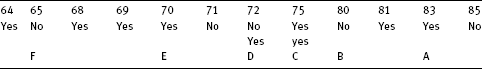
For example, we can discretize the temperature attribute values in the weather data, the value of which is given in Tab. 3.5.
These values correspond to 11 possible separation points, and the information entropy of each point can be calculated in the usual way. For instance, temperature < 71.5 divides the instance into four positive and two negative data, corresponding to five “yes” and three “no” answers. Thus, the information entropy is
This represents the information entropy required to distinguish between individual yes and no values by segmentation. In the process of discretization, the point at which the information entropy is minimized in each operation is selected in order to make the instance class in the interval as simple as possible. The final results are presented in Tab. 3.6.
Tab. 3.5: Attribute values of temperature.

Tab. 3.6: Discretization of temperature.
Although the discretization algorithm based on information entropy is quite successful in some applications, the threshold for the termination of the partitioning process must be set. Therefore, some problems will arise when the interval is partitioned [39]. If a uniform threshold is used for multiple numerical attributes, the number of intervals after attribute discretization will be very different, which may affect the generation of decision tree support rules. An improper choice of the threshold value may also cause the condition attribute value of the original instance after discretization to be the same, as well as giving conflicting data for different decision attribute values (if the condition attribute value of two instances is the same but the decision attribute values are different, the instance set is inconsistent). Therefore, the discretization method based on information entropy lacks operability, and a new method should be developed to make the discretization process simpler, more accurate and more consistent.
4. Discretization method based on dynamic fuzzy partition lattice
The Dynamic Fuzzy Partitioning Lattice was defined in Section 3.2 to discuss the relationship between the partitions of the instance set in the DFDT layers. The Dynamic Fuzzy Partition Lattice divides the finite definite region of the instance set. The range of the numerical attributes is also a definite region, the division of which is limited.
Consider a DFDT where are numeric attributes. To discretize the attributes we must first sort them. The values of are arranged in ascending order, and a separation point is inserted at the interval of the data sequence to obtain a division of