1.4 Process control model of DFMLS

Search in book...
Toggle Font Controls
Create new playlist

Name your new playlist

Playlist description (optional)
Sign In

Email address

Password

Forgot Password?

or

Continue with Facebook

Continue with Google
Sign Up

Full Name

Email address

Confirm Email Address

Password

or

Continue with Facebook

Continue with Google

Assumptions: (1) Response variables are fully observed, with $({\overset{\leftarrow}{y}}_{i}, {\overset{\leftarrow}{y}}_{i})$ $({\overset{\leftarrow}{y}}_{i}, {\overset{\leftarrow}{y}}_{i})$ $| ({\overset{\leftarrow}{x}}_{i}, {\overset{\leftarrow}{x}}_{i}) (i = 1, 2, ..., n)$ $| ({\overset{\leftarrow}{x}}_{i}, {\overset{\leftarrow}{x}}_{i}) (i = 1, 2, ..., n)$ independent mutual conditions. The conditional density function is then $p (({\overset{\leftarrow}{y}}_{i}, {\overset{\leftarrow}{y}}_{i}) | ({\overset{\leftarrow}{x}}_{i}, {\overset{\leftarrow}{x}}_{i})) = a (({\overset{\leftarrow}{y}}_{i}, {\overset{\leftarrow}{y}}_{i}) | {(\overset{\leftarrow}{σ}, \vec{σ})}^{2})$ $p (({\overset{\leftarrow}{y}}_{i}, {\overset{\leftarrow}{y}}_{i}) | ({\overset{\leftarrow}{x}}_{i}, {\overset{\leftarrow}{x}}_{i})) = a (({\overset{\leftarrow}{y}}_{i}, {\overset{\leftarrow}{y}}_{i}) | {(\overset{\leftarrow}{σ}, \vec{σ})}^{2})$ $\exp {- \frac{1}{2 {(\overset{\leftarrow}{σ}, \vec{σ})}^{2}} d_{i} ({\overset{\leftarrow}{y}}_{i}, {\overset{\leftarrow}{y}}_{i}); ({\overset{\leftarrow}{μ}}_{i}, {\vec{μ}}_{t})} (i = 1, 2, ..., n);$ $\exp {- \frac{1}{2 {(\overset{\leftarrow}{σ}, \vec{σ})}^{2}} d_{i} ({\overset{\leftarrow}{y}}_{i}, {\overset{\leftarrow}{y}}_{i}); ({\overset{\leftarrow}{μ}}_{i}, {\vec{μ}}_{t})} (i = 1, 2, ..., n);$

(2) The vector $({\overset{\leftarrow}{x}}_{i}, {\overset{\leftarrow}{x}}_{i}),$ $({\overset{\leftarrow}{x}}_{i}, {\overset{\leftarrow}{x}}_{i}),$ which is composed of k explanatory variables, is a discrete random vector whose distribution density function is $p (({\overset{\leftarrow}{x}}_{i}, {\overset{\leftarrow}{x}}_{i}) | (\overset{\leftarrow}{γ}, \vec{γ})), (\overset{\leftarrow}{γ}, \vec{γ})$ $p (({\overset{\leftarrow}{x}}_{i}, {\overset{\leftarrow}{x}}_{i}) | (\overset{\leftarrow}{γ}, \vec{γ})), (\overset{\leftarrow}{γ}, \vec{γ})$ $= (({\overset{\leftarrow}{γ}}_{1}, {\overset{\leftarrow}{γ}}_{1}), ({\overset{\leftarrow}{γ}}_{2}, {\overset{\leftarrow}{γ}}_{2}), ..., ({\overset{\leftarrow}{γ}}_{r}, {\overset{\leftarrow}{γ}}_{r})) .$ $= (({\overset{\leftarrow}{γ}}_{1}, {\overset{\leftarrow}{γ}}_{1}), ({\overset{\leftarrow}{γ}}_{2}, {\overset{\leftarrow}{γ}}_{2}), ..., ({\overset{\leftarrow}{γ}}_{r}, {\overset{\leftarrow}{γ}}_{r})) .$ Some of the explanatory variable values are missing in the partially observed data points, and this loss is random; $({\overset{\leftarrow}{x}}_{i}, {\overset{\leftarrow}{x}}_{i})$ $({\overset{\leftarrow}{x}}_{i}, {\overset{\leftarrow}{x}}_{i})$ (i = 1, 2, . . ., n) are independent of each other.

Set $(\overset{\leftarrow}{θ}, \vec{θ}) = ({(\overset{\leftarrow}{β}, \vec{β})}^{T}, {(\overset{\leftarrow}{γ}, \vec{γ})}^{T}), Then, (({\overset{\leftarrow}{x}}_{i}, {\overset{\leftarrow}{x}}_{i}) ({\overset{\leftarrow}{y}}_{i}, {\overset{\leftarrow}{y}}_{i}))$ $(\overset{\leftarrow}{θ}, \vec{θ}) = ({(\overset{\leftarrow}{β}, \vec{β})}^{T}, {(\overset{\leftarrow}{γ}, \vec{γ})}^{T}), Then, (({\overset{\leftarrow}{x}}_{i}, {\overset{\leftarrow}{x}}_{i}) ({\overset{\leftarrow}{y}}_{i}, {\overset{\leftarrow}{y}}_{i}))$ is the joint probability density $p (({\overset{\leftarrow}{x}}_{i}, {\overset{\leftarrow}{x}}_{i}), ({\overset{\leftarrow}{y}}_{i}, {\overset{\leftarrow}{y}}_{i})) = p (({\overset{\leftarrow}{x}}_{i}, {\overset{\leftarrow}{x}}_{i}) | ({\overset{\leftarrow}{y}}_{i}, {\overset{\leftarrow}{y}}_{i})) | (\overset{\leftarrow}{γ}, \vec{γ}) .$ $p (({\overset{\leftarrow}{x}}_{i}, {\overset{\leftarrow}{x}}_{i}), ({\overset{\leftarrow}{y}}_{i}, {\overset{\leftarrow}{y}}_{i})) = p (({\overset{\leftarrow}{x}}_{i}, {\overset{\leftarrow}{x}}_{i}) | ({\overset{\leftarrow}{y}}_{i}, {\overset{\leftarrow}{y}}_{i})) | (\overset{\leftarrow}{γ}, \vec{γ}) .$ The joint α-log likelihood function of $(({\overset{\leftarrow}{x}}_{i}, {\overset{\leftarrow}{x}}_{i}), ({\overset{\leftarrow}{y}}_{i}, {\overset{\leftarrow}{y}}_{i}))$ $(({\overset{\leftarrow}{x}}_{i}, {\overset{\leftarrow}{x}}_{i}), ({\overset{\leftarrow}{y}}_{i}, {\overset{\leftarrow}{y}}_{i}))$ is

if we define $L_{({\overset{\leftarrow}{y}}_{i}, {\overset{\leftarrow}{y}}_{i}) | ({\overset{\leftarrow}{x}}_{i}, {\overset{\leftarrow}{x}}_{i})}^{(α)} (\overset{\leftarrow}{β}, \vec{β}) = L^{(α)} (p ({\overset{\leftarrow}{y}}_{i}, {\overset{\leftarrow}{y}}_{i}) | ({\overset{\leftarrow}{x}}_{i}, {\overset{\leftarrow}{x}}_{i})),$ $L_{({\overset{\leftarrow}{y}}_{i}, {\overset{\leftarrow}{y}}_{i}) | ({\overset{\leftarrow}{x}}_{i}, {\overset{\leftarrow}{x}}_{i})}^{(α)} (\overset{\leftarrow}{β}, \vec{β}) = L^{(α)} (p ({\overset{\leftarrow}{y}}_{i}, {\overset{\leftarrow}{y}}_{i}) | ({\overset{\leftarrow}{x}}_{i}, {\overset{\leftarrow}{x}}_{i})),$ then $L_{({\overset{\leftarrow}{x}}_{i}, {\overset{\leftarrow}{x}}_{i})}^{(α)}$ $L_{({\overset{\leftarrow}{x}}_{i}, {\overset{\leftarrow}{x}}_{i})}^{(α)}$ $(\overset{\leftarrow}{γ}, \vec{γ}) = L^{(α)} (p (({\overset{\leftarrow}{x}}_{i}, {\overset{\leftarrow}{x}}_{i}) | (\overset{\leftarrow}{γ}, \vec{γ})))$ $(\overset{\leftarrow}{γ}, \vec{γ}) = L^{(α)} (p (({\overset{\leftarrow}{x}}_{i}, {\overset{\leftarrow}{x}}_{i}) | (\overset{\leftarrow}{γ}, \vec{γ})))$ is the edge α-log likelihood function of $({\overset{\leftarrow}{x}}_{i}, {\overset{\leftarrow}{x}}_{i}) .$ $({\overset{\leftarrow}{x}}_{i}, {\overset{\leftarrow}{x}}_{i}) .$ Thus, the combined α-log likelihood function of $(\overset{\leftarrow}{y}, \overset{\leftarrow}{y}) = (({\overset{\leftarrow}{y}}_{1}, {\overset{\leftarrow}{y}}_{1})),$ $(\overset{\leftarrow}{y}, \overset{\leftarrow}{y}) = (({\overset{\leftarrow}{y}}_{1}, {\overset{\leftarrow}{y}}_{1})),$ $({\overset{\leftarrow}{y}}_{2}, {\overset{\leftarrow}{y}}_{2}), ..., {({\overset{\leftarrow}{y}}_{2}, {\overset{\leftarrow}{y}}_{2})}^{T} and (\overset{\leftarrow}{x}, \vec{x}) = {(({\overset{\leftarrow}{x}}_{1}, {\overset{\leftarrow}{x}}_{1}), ({\overset{\leftarrow}{x}}_{2}, {\overset{\leftarrow}{x}}_{2}), ..., ({\overset{\leftarrow}{x}}_{n}, {\overset{\leftarrow}{x}}_{n}))}^{T}$ $({\overset{\leftarrow}{y}}_{2}, {\overset{\leftarrow}{y}}_{2}), ..., {({\overset{\leftarrow}{y}}_{2}, {\overset{\leftarrow}{y}}_{2})}^{T} and (\overset{\leftarrow}{x}, \vec{x}) = {(({\overset{\leftarrow}{x}}_{1}, {\overset{\leftarrow}{x}}_{1}), ({\overset{\leftarrow}{x}}_{2}, {\overset{\leftarrow}{x}}_{2}), ..., ({\overset{\leftarrow}{x}}_{n}, {\overset{\leftarrow}{x}}_{n}))}^{T}$ can be expressed as

Set the complete data $Unexpected text node: ' x '$ $({\overset{\leftarrow}{x}}_{i}, {\vec{x}}_{i}) = (({\overset{\leftarrow}{x}}_{o b s, i}, {\overset{\leftarrow}{x}}_{o b s, i}), ({\overset{\leftarrow}{x}}_{m i s, i}, {\overset{\leftarrow}{x}}_{m i s, i})), {where(\overset{\leftarrow}{x}}_{o b s, i},$ ${\vec{x}}_{o b s, i})$ ${\vec{x}}_{o b s, i})$ is the observed data of $({\overset{\leftarrow}{x}}_{i}, {\overset{\leftarrow}{x}}_{i}), ({\overset{\leftarrow}{x}}_{m i s, i}, {\overset{\leftarrow}{x}}_{m i s, i})$ $({\overset{\leftarrow}{x}}_{i}, {\overset{\leftarrow}{x}}_{i}), ({\overset{\leftarrow}{x}}_{m i s, i}, {\overset{\leftarrow}{x}}_{m i s, i})$ is the missing data of $({\overset{\leftarrow}{x}}_{i},$ $({\overset{\leftarrow}{x}}_{i},$ ${\overset{\leftarrow}{x}}_{i}), p (({\overset{\leftarrow}{x}}_{m i s, i}, {\overset{\leftarrow}{x}}_{m i s, i}) | ({\overset{\leftarrow}{x}}_{o b s, i}, {\overset{\leftarrow}{x}}_{o b s, i}), ({\overset{\leftarrow}{y}}_{i}, {\vec{y}}_{i}), (\overset{\leftarrow}{θ}, \vec{θ}))$ ${\overset{\leftarrow}{x}}_{i}), p (({\overset{\leftarrow}{x}}_{m i s, i}, {\overset{\leftarrow}{x}}_{m i s, i}) | ({\overset{\leftarrow}{x}}_{o b s, i}, {\overset{\leftarrow}{x}}_{o b s, i}), ({\overset{\leftarrow}{y}}_{i}, {\vec{y}}_{i}), (\overset{\leftarrow}{θ}, \vec{θ}))$ is the conditional distribution density function of the missing explanatory variable $({\overset{\leftarrow}{x}}_{m i s, i}, {\overset{\leftarrow}{x}}_{m i s, i})$ $({\overset{\leftarrow}{x}}_{m i s, i}, {\overset{\leftarrow}{x}}_{m i s, i})$ under the condition of $(\overset{\leftarrow}{θ}, \vec{θ}),$ $(\overset{\leftarrow}{θ}, \vec{θ}),$ and the observed data $({\overset{\leftarrow}{x}}_{o b s, i}, {\overset{\leftarrow}{x}}_{o b s, i})$ $({\overset{\leftarrow}{x}}_{o b s, i}, {\overset{\leftarrow}{x}}_{o b s, i})$ are given.

Thus, the dynamic fuzzy MLE algorithm (dynamic fuzzy α − EM algorithm) is shown in Algorithm 1.3.

Algorithm 1.3 DF α − EM algorithm

Dynamic fuzzy α -E step:

where ${(\overset{\leftarrow}{θ}, \vec{θ})}^{(m)}$ ${(\overset{\leftarrow}{θ}, \vec{θ})}^{(m)}$ denotes the iteration value of $(\overset{\leftarrow}{θ}, \vec{θ})$ $(\overset{\leftarrow}{θ}, \vec{θ})$ obtained by the m th dynamic fuzzy α-EM iteration, E represents the expectation with respect to the distribution $p (({\overset{\leftarrow}{x}}_{m i s, i}, {\overset{\leftarrow}{x}}_{m i s, i})) | ({\overset{\leftarrow}{x}}_{o b s}),$ $p (({\overset{\leftarrow}{x}}_{m i s, i}, {\overset{\leftarrow}{x}}_{m i s, i})) | ({\overset{\leftarrow}{x}}_{o b s}),$ ${\vec{x}}_{o b j, i}), ({\vec{y}}_{i}, {\vec{y}}_{i}), {(\overset{\leftarrow}{θ}, \vec{θ})}^{(m)),} \sum_{({\overset{\leftarrow}{x}}_{m i s, i}, {\overset{\leftarrow}{x}}_{m i s, i})}$ ${\vec{x}}_{o b j, i}), ({\vec{y}}_{i}, {\vec{y}}_{i}), {(\overset{\leftarrow}{θ}, \vec{θ})}^{(m)),} \sum_{({\overset{\leftarrow}{x}}_{m i s, i}, {\overset{\leftarrow}{x}}_{m i s, i})}$ represents the sum of all possible values of the missing explanatory variable $({\overset{\leftarrow}{x}}_{m i s, j}, {\overset{\leftarrow}{x}}_{m i s, j}),$ $({\overset{\leftarrow}{x}}_{m i s, j}, {\overset{\leftarrow}{x}}_{m i s, j}),$ and the conditional distribution density function for the missing explanatory variable $({\overset{\leftarrow}{x}}_{m i s, j}, {\overset{\leftarrow}{x}}_{m i s, j})$ $({\overset{\leftarrow}{x}}_{m i s, j}, {\overset{\leftarrow}{x}}_{m i s, j})$ under the condition of ${(\overset{\leftarrow}{θ}, \vec{θ})}^{m}$ ${(\overset{\leftarrow}{θ}, \vec{θ})}^{m}$ and the observed data $({\overset{\leftarrow}{x}}_{o b s, j})$ $({\overset{\leftarrow}{x}}_{o b s, j})$ ${\vec{x}}_{o b s, i})$ ${\vec{x}}_{o b s, i})$ are given. The Bayesian formula can be directly applied to get:

Dynamic fuzzy α-E step:

and set the sum of the two terms on the right of (1.22) as $Q_{1}^{(α)} ((\overset{\leftarrow}{β}, \vec{β}) | {(\overset{\leftarrow}{θ}, \vec{θ})}^{(m)}), Q_{2}^{(α)} (\overset{\leftarrow}{γ}, \vec{γ}) |$ $Q_{1}^{(α)} ((\overset{\leftarrow}{β}, \vec{β}) | {(\overset{\leftarrow}{θ}, \vec{θ})}^{(m)}), Q_{2}^{(α)} (\overset{\leftarrow}{γ}, \vec{γ}) |$ ${(\overset{\leftarrow}{θ}, \vec{θ})}^{(m)}),$ ${(\overset{\leftarrow}{θ}, \vec{θ})}^{(m)}),$ respectively. Because $Q_{1}^{(a)} ((\overset{\leftarrow}{β}, \vec{β}) | {(\overset{\leftarrow}{θ}, \vec{θ})}^{(m)}), Q_{2}^{(a)} ((\overset{\leftarrow}{γ}, \vec{γ}) | {(\overset{\leftarrow}{θ}, \vec{θ})}^{(m)})$ $Q_{1}^{(a)} ((\overset{\leftarrow}{β}, \vec{β}) | {(\overset{\leftarrow}{θ}, \vec{θ})}^{(m)}), Q_{2}^{(a)} ((\overset{\leftarrow}{γ}, \vec{γ}) | {(\overset{\leftarrow}{θ}, \vec{θ})}^{(m)})$ are non-negative, the (m + 1)th dynamic ambiguity α-EM iteration can be transformed to:

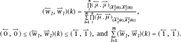
The method of solving ${(\overset{\leftarrow}{γ}, \vec{γ})}^{(m + 1)}$ ${(\overset{\leftarrow}{γ}, \vec{γ})}^{(m + 1)}$ is related to the distribution of the explanatory variables. The iterative formula for solving is [32]:

the definition of each variable is described in [32].

The above two steps are repeated until convergence.

1.3.2.2Convergence of algorithms

We will describe the convergence behaviour of the convergence of is similar.

Theorem 1.6

Theorem 1.7 is monotonically increasing [28].

Theorem 1.8 Let be continuous in and differentiable in its interior [29]. For any if the set is dense and is inside holds for all and m. Then, we have the following conclusions:

(1)The limit point of the sequence is the fixed point of

(2) converges monotonically to

Proof: Define the iterative operator:

Under the conditions of the theorem, the operator Λ(α) is closed.

inside guarantees that and are differentiable for any such that the global convergence conditions in [30] and [31] are satisfied:

(1)Sequence is generated by

(2)The fixed point set of the iterative operator Λ(α) is contained in a dense set

(3) is continuous. Thus, for there is

Therefore, by the global convergence theorem in [30] and [31], the proof is complete.

1.3.2.3Examples

Table 1.1 provides complete data for 32 patients with haematological malignancy, from Ibrahim (1900). Assume that the 3rd, 8th, 19th, 27th, and 32nd data points are not fully observed, see Tab. 1.2, which is taken from [32]. In the table, t represents the patient’s duration (weeks); indicates that a biological characteristic test for leukocytes is positive, indicates that the test was negative; z = 0 indicates that there are less than 11,000 white blood cells in the blood to be tested, z = 1 represents 11,000 ≤ WBC ≤ 40,000, and z = 2 represents WBC > 40,000.

Variable z has three states. Therefore, two dummy dynamic fuzzy variables are introduced. When

Assuming that follows the parameter and the logarithmic gamma distribution of the mean then

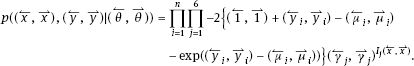
Suppose the joint probability distribution of denotes the function of the j th result of is the probability corresponding to the j th result of Setting the probability density of the complete data based on n= 32 observation points of can be expressed as

Tab. 1.1: Blood cancer patient data.

Tab. 1.2: Partially incomplete data.

The probability density of the incomplete data is

The α – log likelihood ratio of the complete data is

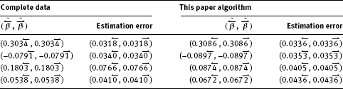
Our basic task is to estimate the parameter Table 1.3 gives only the maximum likelihood estimate and the estimated standard error, which is the same as the EM algorithm in [32]. However, the convergence speed is different. The influence of different α on the convergence rate indicator can be ascertained from Tab. 1.4. When α = − 1, we have the EM algorithm. Obviously, obtaining the appropriate of the parameter will greatly improve the convergence rate of the algorithm, overcoming the shortcoming of the EM algorithm [29]; of course, which value of α gives the fastest convergence speed requires further exploration.

Note: In Tab. 1.4, the CPU time ratio is the ratio of the CPU consumed by the algorithm to the time taken to execute the algorithm; the CPU time rate is the number of time cycles of the algorithm that the CPU executes per unit of time and the number of time periods of the CPU itself.

Tab. 1.3: Numerical test results.

Tab. 1.4: Effect of α on the convergence rate index.

1.4Process control model of DFMLS [8]

Studying the visualization and process control of machine learning is a fundamental problem. This section attempts to examine this issue from the perspective of process control to study the problem of learning. The results are summarized below.

1.4.1Process control model of DFMLS

For a DFMLS composed of m rules Rl(l = 1, 2, . . ., m), the global model of the system is

As each dynamic fuzzy subsystem is linearly descriptive, when we choose the global dynamic fuzzy control law, we first use linear system theory to stabilize the subsystem and obtain the local dynamic fuzzy control law that satisfies the subsystem design requirements. The global dynamic fuzzy control law is a weighted combination of subsystem control laws.

The dynamic fuzzy control rules are as follows:

and the global control is

Thus, the global model of the DFML process control system (hereinafter referred to as dynamic fuzzy control system) is

For ease of analysis, note that

1.4.2Stability analysis

The most important characteristic of the control system is its stability, because an unstable system is unable to complete the expected control tasks. This section presents a stability analysis of the dynamic fuzzy control system.

Theorem 1.9 For the dynamic fuzzy control system shown in (1.26), if there exists a common dynamic fuzzy positive definite matrix such that [33]

is valid, then the dynamic fuzzy control system (1.26) is globally asymptotically stable.

In general, even if all the subsystems are stable, there is a possibility that the public dynamic fuzzy positive definite matrix $(\overset{↼}{P}, \overset{⇀}{P})$ $(\overset{↼}{P}, \overset{⇀}{P})$ does not exist, so that (1.28) holds, especially when dynamic fuzzy control rules are more difficult to apply or are invalid [34]. To avoid the difficulty of finding $(\overset{↼}{P}, \overset{⇀}{P}),$ $(\overset{↼}{P}, \overset{⇀}{P}),$ we propose a simple and effective method to judge the stability of closed-loop dynamic fuzzy control systems based on the interval matrix and robust control theory.

$(\overset{↼}{C}, \overset{⇀}{C})$ $(\overset{↼}{C}, \overset{⇀}{C})$ changes with the state value $(\overset{↼}{X}, \overset{⇀}{X}) (k)$ $(\overset{↼}{X}, \overset{⇀}{X}) (k)$ at each time, but any element $({\overset{↼}{c}}_{i j}, {\overset{⇀}{c}}_{i j}) in (\overset{↼}{C}, \overset{⇀}{C})$ $({\overset{↼}{c}}_{i j}, {\overset{⇀}{c}}_{i j}) in (\overset{↼}{C}, \overset{⇀}{C})$ is the weighted sum of the corresponding elements of the subsystem. Thus, we know that the elements of $(\overset{↼}{C}, \overset{⇀}{C})$ $(\overset{↼}{C}, \overset{⇀}{C})$ are in the determined closed interval given by $(\overset{↼}{C}, \overset{⇀}{C}) \max = \max_{l} ({\overset{↼}{c}}_{i j}^{l}, {\overset{⇀}{c}}_{i j}^{l}), {(\overset{↼}{C}, \overset{⇀}{C})}_{\min} = \min_{l} ({\overset{↼}{c}}_{i j}^{l}, {\overset{↼}{c}}_{i j}^{l}) . Then (\overset{↼}{C}, \overset{⇀}{C}) \in$ $(\overset{↼}{C}, \overset{⇀}{C}) \max = \max_{l} ({\overset{↼}{c}}_{i j}^{l}, {\overset{⇀}{c}}_{i j}^{l}), {(\overset{↼}{C}, \overset{⇀}{C})}_{\min} = \min_{l} ({\overset{↼}{c}}_{i j}^{l}, {\overset{↼}{c}}_{i j}^{l}) . Then (\overset{↼}{C}, \overset{⇀}{C}) \in$ $[{(\overset{↼}{C}, \overset{⇀}{C})}_{\min}, {(\overset{↼}{C}, \overset{⇀}{C})}_{\max}], Write ({\overset{↼}{C}}_{0}, {\overset{⇀}{C}}_{0}) = ({(\overset{↼}{C}, \overset{⇀}{C})}_{\max} + {(\overset{↼}{C}, \overset{⇀}{C})}_{\min}) / 2, (\overset{↼}{H}, \overset{⇀}{H}) =$ $[{(\overset{↼}{C}, \overset{⇀}{C})}_{\min}, {(\overset{↼}{C}, \overset{⇀}{C})}_{\max}], Write ({\overset{↼}{C}}_{0}, {\overset{⇀}{C}}_{0}) = ({(\overset{↼}{C}, \overset{⇀}{C})}_{\max} + {(\overset{↼}{C}, \overset{⇀}{C})}_{\min}) / 2, (\overset{↼}{H}, \overset{⇀}{H}) =$ $({(\overset{↼}{C}, \overset{⇀}{C})}_{\max} - {(\overset{↼}{C}, \overset{⇀}{C})}_{\min}) / 2 (\overset{↼}{H}, \overset{⇀}{H}) = (({\overset{↼}{h}}_{i j}, {\overset{⇀}{h}}_{i j})) .$ $({(\overset{↼}{C}, \overset{⇀}{C})}_{\max} - {(\overset{↼}{C}, \overset{⇀}{C})}_{\min}) / 2 (\overset{↼}{H}, \overset{⇀}{H}) = (({\overset{↼}{h}}_{i j}, {\overset{⇀}{h}}_{i j})) .$

Using the properties of interval matrices, $(\overset{↼}{C}, \overset{⇀}{C})$ $(\overset{↼}{C}, \overset{⇀}{C})$ can be equivalently expressed as follows:

where

Here, $({\overset{↼}{e}}_{i}, {\overset{⇀}{e}}_{i})$ $({\overset{↼}{e}}_{i}, {\overset{⇀}{e}}_{i})$ is the unit dynamic fuzzy column vector whose i th element is $(\overset{↼}{1}, \overset{⇀}{1}),$ $(\overset{↼}{1}, \overset{⇀}{1}),$ and the remaining elements are $(\overset{↼}{0}, \overset{⇀}{0}); (\overset{↼}{M}, \overset{⇀}{M}) ϵ {(\overset{↼}{R}, \overset{⇀}{R})}^{n \times n^{2}}, (\overset{↼}{N}, \overset{⇀}{N}) ϵ {(\overset{↼}{R}, \overset{⇀}{R})}^{h n^{2} \times n},$ $(\overset{↼}{0}, \overset{⇀}{0}); (\overset{↼}{M}, \overset{⇀}{M}) ϵ {(\overset{↼}{R}, \overset{⇀}{R})}^{n \times n^{2}}, (\overset{↼}{N}, \overset{⇀}{N}) ϵ {(\overset{↼}{R}, \overset{⇀}{R})}^{h n^{2} \times n},$ $(\overset{↼}{Σ}, \overset{⇀}{Σ}) ϵ {(\overset{↼}{R}, \overset{⇀}{R})}^{n^{2} \times n^{2}}$ $(\overset{↼}{Σ}, \overset{⇀}{Σ}) ϵ {(\overset{↼}{R}, \overset{⇀}{R})}^{n^{2} \times n^{2}}$ is the dynamic fuzzy diagonal matrix, and the value of $(\overset{↼}{Σ}, \overset{⇀}{Σ})$ $(\overset{↼}{Σ}, \overset{⇀}{Σ})$ changes with the rule weight value at each time, but ${(\overset{↼}{Σ}, \overset{⇀}{Σ})}^{T} (k) (\overset{↼}{Σ}, \overset{⇀}{Σ}) (k) \leq (\overset{↼}{I}, \overset{⇀}{I}) .$ ${(\overset{↼}{Σ}, \overset{⇀}{Σ})}^{T} (k) (\overset{↼}{Σ}, \overset{⇀}{Σ}) (k) \leq (\overset{↼}{I}, \overset{⇀}{I}) .$ Then, the global model of the closed-loop dynamic fuzzy control system can be expressed as

Definition 1.10 For an uncertain dynamic fuzzy autonomous system [35],

$\begin{array}{l} | ({\overset{↼}{ε}}_{i j}, {\overset{⇀}{ε}}_{i j}) (k) | \leq (\overset{↼}{1}, \overset{⇀}{1}), (i, j) = 1, 2, ..., n; \\ (\overset{↼}{M}, \overset{⇀}{M}) = [\sqrt{({\overset{↼}{h}}_{11}, {\overset{⇀}{h}}_{11})} ({\overset{↼}{e}}_{1}, {\overset{⇀}{e}}_{1}) ... \sqrt{({\overset{↼}{h}}_{1 N}, {\overset{⇀}{h}}_{1 n})} ({\overset{↼}{e}}_{1}, {\overset{⇀}{e}}_{1}) ... \sqrt{({\overset{↼}{h}}_{N 1}, {\overset{⇀}{h}}_{n 1})} ({\overset{↼}{e}}_{n}, {\overset{⇀}{e}}_{n}) \\ \sqrt{({\overset{↼}{h}}_{n n}, {\overset{⇀}{h}}_{n n})} ({\overset{↼}{e}}_{N}, {\overset{↼}{e}}_{N})] \\ (\overset{↼}{N}, \overset{⇀}{N}) = [\sqrt{({\overset{↼}{h}}_{11}, {\overset{⇀}{h}}_{11})} ({\overset{↼}{e}}_{1}, {\overset{⇀}{e}}_{1}) ... \sqrt{({\overset{↼}{h}}_{1 N}, {\overset{⇀}{h}}_{1 n})} ({\overset{↼}{e}}_{n}, {\overset{⇀}{e}}_{n}) ... \sqrt{({\overset{↼}{h}}_{n 1}, {\overset{⇀}{h}}_{N 1})} ({\overset{↼}{e}}_{1}, {\overset{⇀}{e}}_{1}) ... \\ {\sqrt{({\overset{↼}{h}}_{n n}, {\overset{⇀}{h}}_{n n})} ({\overset{↼}{e}}_{N}, {\overset{↼}{e}}_{N})]}^{T} . \end{array}$ $\begin{array}{l} | ({\overset{↼}{ε}}_{i j}, {\overset{⇀}{ε}}_{i j}) (k) | \leq (\overset{↼}{1}, \overset{⇀}{1}), (i, j) = 1, 2, ..., n; \\ (\overset{↼}{M}, \overset{⇀}{M}) = [\sqrt{({\overset{↼}{h}}_{11}, {\overset{⇀}{h}}_{11})} ({\overset{↼}{e}}_{1}, {\overset{⇀}{e}}_{1}) ... \sqrt{({\overset{↼}{h}}_{1 N}, {\overset{⇀}{h}}_{1 n})} ({\overset{↼}{e}}_{1}, {\overset{⇀}{e}}_{1}) ... \sqrt{({\overset{↼}{h}}_{N 1}, {\overset{⇀}{h}}_{n 1})} ({\overset{↼}{e}}_{n}, {\overset{⇀}{e}}_{n}) \\ \sqrt{({\overset{↼}{h}}_{n n}, {\overset{⇀}{h}}_{n n})} ({\overset{↼}{e}}_{N}, {\overset{↼}{e}}_{N})] \\ (\overset{↼}{N}, \overset{⇀}{N}) = [\sqrt{({\overset{↼}{h}}_{11}, {\overset{⇀}{h}}_{11})} ({\overset{↼}{e}}_{1}, {\overset{⇀}{e}}_{1}) ... \sqrt{({\overset{↼}{h}}_{1 N}, {\overset{⇀}{h}}_{1 n})} ({\overset{↼}{e}}_{n}, {\overset{⇀}{e}}_{n}) ... \sqrt{({\overset{↼}{h}}_{n 1}, {\overset{⇀}{h}}_{N 1})} ({\overset{↼}{e}}_{1}, {\overset{⇀}{e}}_{1}) ... \\ {\sqrt{({\overset{↼}{h}}_{n n}, {\overset{⇀}{h}}_{n n})} ({\overset{↼}{e}}_{N}, {\overset{↼}{e}}_{N})]}^{T} . \end{array}$

if there exists an n-order dynamic fuzzy positive definite matrix $(\overset{↼}{P}, \overset{⇀}{P})$ $(\overset{↼}{P}, \overset{⇀}{P})$ and a dynamic fuzzy constant $(\overset{↼}{α}, \overset{⇀}{α}) > (\overset{↼}{0}, \overset{⇀}{0})$ $(\overset{↼}{α}, \overset{⇀}{α}) > (\overset{↼}{0}, \overset{⇀}{0})$ such that, for any permissible uncertainty $Δ (\overset{↼}{A}, \overset{⇀}{A}),$ $Δ (\overset{↼}{A}, \overset{⇀}{A}),$

$(\overset{↼}{X}, \overset{⇀}{X}) (t) = (({\overset{↼}{A}}_{0}, {\overset{⇀}{A}}_{0}) + Δ (\overset{↼}{A}, \overset{⇀}{A})) (\overset{↼}{X}, \overset{⇀}{X}) (t),$ $(\overset{↼}{X}, \overset{⇀}{X}) (t) = (({\overset{↼}{A}}_{0}, {\overset{⇀}{A}}_{0}) + Δ (\overset{↼}{A}, \overset{⇀}{A})) (\overset{↼}{X}, \overset{⇀}{X}) (t),$

holds for any solution $(\overset{↼}{X}, \overset{⇀}{X}) (t)$ $(\overset{↼}{X}, \overset{⇀}{X}) (t)$ and t, then the system is said to be quadratic stable. In the above expression, $({\overset{↼}{A}}_{0}, {\overset{⇀}{A}}_{0}) = ({(\overset{↼}{A}, \overset{⇀}{A})}_{\max} + {(\overset{↼}{A}, \overset{⇀}{A})}_{\min}) / 2 {(\overset{↼}{A}, \overset{⇀}{A})}_{\max} =$ $({\overset{↼}{A}}_{0}, {\overset{⇀}{A}}_{0}) = ({(\overset{↼}{A}, \overset{⇀}{A})}_{\max} + {(\overset{↼}{A}, \overset{⇀}{A})}_{\min}) / 2 {(\overset{↼}{A}, \overset{⇀}{A})}_{\max} =$ $\max_{l} (({\overset{↼}{a}}_{i j}^{l}, {\overset{⇀}{a}}_{i j}^{l})) {(\overset{↼}{A}, \overset{⇀}{A})}_{\min} = \min_{l} (({\overset{↼}{a}}_{i j}^{l}, {\overset{⇀}{a}}_{i j}^{l})) .$ $\max_{l} (({\overset{↼}{a}}_{i j}^{l}, {\overset{⇀}{a}}_{i j}^{l})) {(\overset{↼}{A}, \overset{⇀}{A})}_{\min} = \min_{l} (({\overset{↼}{a}}_{i j}^{l}, {\overset{⇀}{a}}_{i j}^{l})) .$

..................Content has been hidden....................

You can't read the all page of ebook, please click here login for view all page.

Table of Contents for 1.4 Process control model of DFMLS

Create new playlist

Sign In

Sign Up

1.3.2.2Convergence of algorithms

1.3.2.3Examples

1.4Process control model of DFMLS [8]

1.4.1Process control model of DFMLS

1.4.2Stability analysis

Table of Contents for
1.4 Process control model of DFMLS