5.6 Summary

Search in book...
Toggle Font Controls
Create new playlist

Name your new playlist

Playlist description (optional)
Sign In

Email address

Password

Forgot Password?

or

Continue with Facebook

Continue with Google
Sign Up

Full Name

Email address

Confirm Email Address

Password

or

Continue with Facebook

Continue with Google

(2)i2k, a represents the distance between the value $(x^{a}, x^{a})$ $(x^{a}, x^{a})$ of pattern $(\overset{\leftarrow}{x}, \vec{x})$ $(\overset{\leftarrow}{x}, \vec{x})$ on attribute $(\overset{\leftarrow}{a}, \vec{a})$ $(\overset{\leftarrow}{a}, \vec{a})$ and the centre of gravity $({\overset{\leftarrow}{G}}_{k, c u r}^{a}, {\overset{\leftarrow}{G}}_{k, c u r}^{a})$ $({\overset{\leftarrow}{G}}_{k, c u r}^{a}, {\overset{\leftarrow}{G}}_{k, c u r}^{a})$ of the class according to the standard deviation $({\overset{\leftarrow}{S t d}}_{k, c u r}^{a}, {\overset{\leftarrow}{S t d}}_{k, c u r}^{a})$ $({\overset{\leftarrow}{S t d}}_{k, c u r}^{a}, {\overset{\leftarrow}{S t d}}_{k, c u r}^{a})$ of the current category $({\overset{\leftarrow}{C}}_{k}, {\vec{C}}_{k}) .$ $({\overset{\leftarrow}{C}}_{k}, {\vec{C}}_{k}) .$ This is calculated by (5.19). If at least one value of attribute $(\overset{\leftarrow}{a}, \vec{a})$ $(\overset{\leftarrow}{a}, \vec{a})$ is greater than th1, then this pattern will not be in the same region as the other patterns in class $({\overset{\leftarrow}{C}}_{k}, {\vec{C}}_{k}) .$ $({\overset{\leftarrow}{C}}_{k}, {\vec{C}}_{k}) .$

$i_{k, a}^{2} = \frac{| (\overset{\leftarrow}{x^{a}}, {\vec{x}}^{a}) - ({\overset{\leftarrow}{G}}_{k, c u r}^{a}, {\vec{G}}_{k, c u r}^{a}) |}{({\overset{\leftarrow}{S t d}}_{k, c u r}^{a}, {\vec{S t d}}_{k, c u r}^{a})} - (\overset{\leftarrow}{100}, \vec{100}) (5.19)$ $i_{k, a}^{2} = \frac{| (\overset{\leftarrow}{x^{a}}, {\vec{x}}^{a}) - ({\overset{\leftarrow}{G}}_{k, c u r}^{a}, {\vec{G}}_{k, c u r}^{a}) |}{({\overset{\leftarrow}{S t d}}_{k, c u r}^{a}, {\vec{S t d}}_{k, c u r}^{a})} - (\overset{\leftarrow}{100}, \vec{100}) (5.19)$

Note that noise sometimes changes the centre of gravity of the category and the standard deviation, so we need to add an additional constraint: If at least Nk, min consecutive patterns in class $({\overset{\leftarrow}{C}}_{k}, {\vec{C}}_{k})$ $({\overset{\leftarrow}{C}}_{k}, {\vec{C}}_{k})$ are found to be deductive, then we can confirm that the category is deduced. If Nk, min is too large, the detection of the class evolution will be delayed, and we can determine the value of Nk, min according to the ratio of the noise in the pattern and the need to delay the evolution of the detection category. When two successive deductions indicate that the values of i1k, and i2k, are greater than th1, we ensure that the category has been deduced, then adjust the category characteristics as described below.

3) Adjustment of the category characteristics

When class changes are detected in the classification stage, the class characteristics may need to be adjusted. When the category is identified by deduction, the useful model can be employed to create a new category. If there are now c categories, we adjust the class characteristics by the following steps.

(1)Create a new category $({\overset{\leftarrow}{C}}_{k + 1}, {\vec{C}}_{k + 1})$ $({\overset{\leftarrow}{C}}_{k + 1}, {\vec{C}}_{k + 1})$ and select the most representative model for deduction. $(\overset{\leftarrow}{x}, \vec{x})$ $(\overset{\leftarrow}{x}, \vec{x})$ and its k – 1 neighbours are new members of the new class, as the last sample to be classified in class $(\overset{\leftarrow}{x}, \vec{x})$ $(\overset{\leftarrow}{x}, \vec{x})$ is one of the patterns in which the class was deduced. Because the neighbours are already known at the time of class $(\overset{\leftarrow}{x}, \vec{x})$ $(\overset{\leftarrow}{x}, \vec{x})$ there is no need to determine these neighbours by calculating the distance. In short, the k selected nodes constitute the new model of the new category.

(2)The selected pattern is deleted from the original category $({\overset{\leftarrow}{C}}_{i}, {\vec{C}}_{i}),$ $({\overset{\leftarrow}{C}}_{i}, {\vec{C}}_{i}),$ and its new centre of gravity $({\overset{\leftarrow}{G}}_{i, c u r}^{a}, {\vec{G}}_{i, c u r}^{a})$ $({\overset{\leftarrow}{G}}_{i, c u r}^{a}, {\vec{G}}_{i, c u r}^{a})$ and current standard deviation $({\overset{\leftarrow}{S t d}}_{k, c u r}^{a}, {\vec{S t d}}_{k, c u r}^{a})$ $({\overset{\leftarrow}{S t d}}_{k, c u r}^{a}, {\vec{S t d}}_{k, c u r}^{a})$ are calculated.

(3)Calculate the centre of gravity $({\overset{\leftarrow}{G}}_{c + 1, c u r}^{a}, {\vec{G}}_{c + 1, c u r}^{a})$ $({\overset{\leftarrow}{G}}_{c + 1, c u r}^{a}, {\vec{G}}_{c + 1, c u r}^{a})$ and standard deviation $({\overset{\leftarrow}{S t d}}_{c + 1, c u r}^{a}, {\vec{S t d}}_{c + 1, c u r}^{a})$ $({\overset{\leftarrow}{S t d}}_{c + 1, c u r}^{a}, {\vec{S t d}}_{c + 1, c u r}^{a})$ of the new category, and update the total number of cate gories.

4) Determine the class validity

Because noise is present in the training set, if a noise category is created, it should be removed during the validity phase. Categories that are deduced from one state to another are useless and should be removed to avoid excessive growth of the dataset. Category deletion is required when the following situations occur:

(1)A category contains a small number of models, only slightly larger than k, that is, the number of categories is n1 > k;

(2)No new schema has been added to the category to be deleted, but there are enough n2 patterns to appear in the other categories.

Sometimes, instead of deleting categories, similar categories should be merged. In fact, it is necessary to measure the coverage over time of existing categories and those that are created. If multiple categories have been created and the deductions for these new categories tend to be similar, then these categories should be merged. To determine the similarity between two categories for merging, a similarity measure based on fuzzy sets is used [53]. To deal with the dynamic fuzzy problem, we will use the similarity measure based on dynamic fuzzy sets, as shown in (5.20), which takes into account the degree of coverage between categories based on the membership of the classified model. Let $({\overset{\leftarrow}{C}}_{i} (\overset{\leftarrow}{x}), {\vec{C}}_{i} (\vec{x})) and ({\overset{\leftarrow}{C}}_{z} (\overset{\leftarrow}{x}) {\overset{\leftarrow}{C}}_{z} (\vec{x}))$ $({\overset{\leftarrow}{C}}_{i} (\overset{\leftarrow}{x}), {\vec{C}}_{i} (\vec{x})) and ({\overset{\leftarrow}{C}}_{z} (\overset{\leftarrow}{x}) {\overset{\leftarrow}{C}}_{z} (\vec{x}))$ be the memberships of pattern $(\overset{\leftarrow}{x}, \vec{x}),$ $(\overset{\leftarrow}{x}, \vec{x}),$ which belongs to category $({\overset{\leftarrow}{C}}_{i}, {\vec{C}}_{i}) and ({\overset{\leftarrow}{C}}_{z}, {\vec{C}}_{z}),$ $({\overset{\leftarrow}{C}}_{i}, {\vec{C}}_{i}) and ({\overset{\leftarrow}{C}}_{z}, {\vec{C}}_{z}),$ respectively, and let $({\overset{\leftarrow}{δ}}_{i, z}, {\vec{δ}}_{i, z})$ $({\overset{\leftarrow}{δ}}_{i, z}, {\vec{δ}}_{i, z})$ be the similarity between the two categories. Values closer to $(\overset{\leftarrow}{1}, \vec{1})$ $(\overset{\leftarrow}{1}, \vec{1})$ indicate that these two categories are more similar, but we do not need to wait until $({\overset{\leftarrow}{δ}}_{i, z}, {\vec{δ}}_{i, z}) = (\overset{\leftarrow}{1}, \vec{1}) before merging ({\overset{\leftarrow}{C}}_{i}, {\vec{C}}_{i}) and ({\overset{\leftarrow}{C}}_{z}, {\vec{C}}_{z}) .$ $({\overset{\leftarrow}{δ}}_{i, z}, {\vec{δ}}_{i, z}) = (\overset{\leftarrow}{1}, \vec{1}) before merging ({\overset{\leftarrow}{C}}_{i}, {\vec{C}}_{i}) and ({\overset{\leftarrow}{C}}_{z}, {\vec{C}}_{z}) .$ We can merge two categories of operations when the similarity is above a certain threshold of $({\overset{\leftarrow}{δ}}_{i, z}, {\vec{δ}}_{i, z}) .$ $({\overset{\leftarrow}{δ}}_{i, z}, {\vec{δ}}_{i, z}) .$

1. DFSSMTAL algorithm

The Mahalanobis distance metric is an important parameter in both the DFKNN algorithm and the DFSSAL algorithm. Many scholars have proposed various methods of estimating the Mahalanobis distance in order to calculate the distance between samples in KNN classification. There are three main categories [55]: eigenvector methods, convex optimization methods, and neighbour component analysis methods.

Eigenvector methods are often used to solve the linear transformation of the input space. As mentioned in Section 4.1, the Mahalanobis distance metric can be obtained by a linear transformation. Principal component analysis, linear discriminant analysis, and correlation analysis are common feature vector methods. The convex optimization method formalizes distance metric learning as the convex optimization of the key positive semidefinite matrix M. Nearest neighbour component analysis [60] is a novel supervised learning algorithm proposed by Goldberger et al. [6]. To reduce the misclassification rate, the classifier uses the Mahalanobis distance metric as a parameter; that is, the expected misclassification rate is reduced by estimating the linear transformation matrix L. In this section, we discuss how to study the Mahalanobis distance metric from the perspective of DFSSMTL.

1) Mahalanobis distance measurement for single task learning

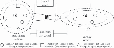
For a single task, the KNNs of a sample X are labelled with the same category using the trained Mahalanobis distance, and differently labelled samples are separated from X. We call the samples with different labels the pseudo-neighbours of X, and those with the same label as sample X are the target neighbours. Assuming that the sample is a target neighbourhood of the sample, it is a pseudo-neighbourhood of the sample, and the learned Markov metric is combined with a larger interval such that each input sample is closer to its target neighbourhood than its pseudo-neighbourhood. The following linear inequality describes this relationship:

$d_{M}^{2} (({\overset{\leftarrow}{x}}_{i}, {\vec{x}}_{i}), ({\overset{\leftarrow}{x}}_{k}, {\vec{x}}_{k})) - d_{M}^{2} (({\overset{\leftarrow}{x}}_{i}, {\vec{x}}_{i}), ({\overset{\leftarrow}{x}}_{j}, {\vec{x}}_{j})) \geq 1 (5.21)$ $d_{M}^{2} (({\overset{\leftarrow}{x}}_{i}, {\vec{x}}_{i}), ({\overset{\leftarrow}{x}}_{k}, {\vec{x}}_{k})) - d_{M}^{2} (({\overset{\leftarrow}{x}}_{i}, {\vec{x}}_{i}), ({\overset{\leftarrow}{x}}_{j}, {\vec{x}}_{j})) \geq 1 (5.21)$

As shown in Fig. 5.10, all samples on the circle are close to sample E and can be the KNNs of sample X. Under the influence of the Mahalanobis distance, the circle becomes elliptical, so that the pseudo-neighbour point and the target neighbourhood point of sample X become larger (K = 3) at the same time.

Fig. 5.10: The changes in neighbourhood of sample X before and after the calculation of Mahalanobis distance.

2) Mahalanobis distance measurement in multi-task background

Assuming that there are T tasks, the training data in each task consist of unlabelled data and tagged data, and the training dataset for the t th task is written as

${(\overset{\leftarrow}{X}, \vec{X})}_{t} = {({(\overset{\leftarrow}{x}, {\vec{x}}_{1})}_{t}, {({\overset{\leftarrow}{y}}_{1}, {\vec{y}}_{1})}_{t}), \dots, ({({\overset{\leftarrow}{x}}_{l}, {\vec{x}}_{l})}_{t}, {({\overset{\leftarrow}{y}}_{l}, {\vec{y}}_{l})}_{t}), {({\overset{\leftarrow}{x}}_{1}, x_{1}^{'})}_{t}, \dots, ({\overset{\leftarrow}{x}}_{u}^{'}, {\vec{x}}_{u}^{'})},$ ${(\overset{\leftarrow}{X}, \vec{X})}_{t} = {({(\overset{\leftarrow}{x}, {\vec{x}}_{1})}_{t}, {({\overset{\leftarrow}{y}}_{1}, {\vec{y}}_{1})}_{t}), \dots, ({({\overset{\leftarrow}{x}}_{l}, {\vec{x}}_{l})}_{t}, {({\overset{\leftarrow}{y}}_{l}, {\vec{y}}_{l})}_{t}), {({\overset{\leftarrow}{x}}_{1}, x_{1}^{'})}_{t}, \dots, ({\overset{\leftarrow}{x}}_{u}^{'}, {\vec{x}}_{u}^{'})},$

where ((xi, xi), (yi, yi) denotes the i th tag data ${({\overset{\leftarrow}{x}}_{i}, {\vec{x}}_{i})}_{t},$ ${({\overset{\leftarrow}{x}}_{i}, {\vec{x}}_{i})}_{t},$ in the t th task, ${({\overset{\leftarrow}{y}}_{i}, {\vec{y}}_{i})}_{t}$ ${({\overset{\leftarrow}{y}}_{i}, {\vec{y}}_{i})}_{t}$ denotes the i th unmarked data of the t th task, lt denotes the number of tag data of the t th task, and ut denotes the number of untagged data for t tasks. The main goal of the DFSSMTAL algorithm is to learn a metric for each task (the metric of the Mahalanobis distance that is learned by the first task is denoted by dMt(⋅,⋅). Then, the task can be learned through DFSSAL. Similar points for all tasks are modelled using the Mahalanobis distance dM0(⋅,⋅), which is shared by all tasks, and the Mahalanobis distance dM0(⋅,⋅) is calculated from the matrix of semi-definite matrices M0. The Mahalanobis distance of each task preserves the individual properties of each task, with the Mahalanobis distance metric for the t th task denoted by dMt(⋅, ⋅) and calculated from the semi-definite matrix Mt. The Mahalanobis distance defining the t th task is given by the following equation:

$d_{M t} ((\overset{\leftarrow}{x}, \vec{x}), (\overset{\leftarrow}{z}, \vec{z})) = \sqrt{{((\overset{\leftarrow}{x}, \vec{x}) - (\overset{\leftarrow}{z}, \vec{z}))}^{T} (M_{0} + M_{t}) ((\overset{\leftarrow}{x}, \vec{x}) - (\overset{\leftarrow}{z}, \vec{z}))} (5.22)$ $d_{M t} ((\overset{\leftarrow}{x}, \vec{x}), (\overset{\leftarrow}{z}, \vec{z})) = \sqrt{{((\overset{\leftarrow}{x}, \vec{x}) - (\overset{\leftarrow}{z}, \vec{z}))}^{T} (M_{0} + M_{t}) ((\overset{\leftarrow}{x}, \vec{x}) - (\overset{\leftarrow}{z}, \vec{z}))} (5.22)$

As shown in Fig. 5.11, M0 grasps the overall trend of the task data, whereas Mt reflects specific tasks.

Before the DFSSMTAL algorithm is presented, we introduce some notations:

(1)(j → i) indicates that sample ${({\overset{\leftarrow}{x}}_{j}, {\vec{x}}_{j})}_{t}$ ${({\overset{\leftarrow}{x}}_{j}, {\vec{x}}_{j})}_{t}$ of the t th task is a target neighbour of sample ${({\overset{\leftarrow}{x}}_{i}, {\vec{x}}_{i})}_{t} .$ ${({\overset{\leftarrow}{x}}_{i}, {\vec{x}}_{i})}_{t} .$

Fig. 5.11: Effects of Mahalanobis distance measurements on nearest neighbours of sample.

(2)(k → i) indicates that sample ${({\overset{\leftarrow}{x}}_{k}, {\vec{x}}_{k})}_{t}$ ${({\overset{\leftarrow}{x}}_{k}, {\vec{x}}_{k})}_{t}$ of the t th task is in the pseudo- neighbourhood of sample ${({\overset{\leftarrow}{x}}_{i}, {\vec{x}}_{i})}_{t} .$ ${({\overset{\leftarrow}{x}}_{i}, {\vec{x}}_{i})}_{t} .$

(3) $S_{t} = {{(i, j, k)}_{t} | {(j \to i)}_{t}, {(k \to i)}_{t}}$ $S_{t} = {{(i, j, k)}_{t} | {(j \to i)}_{t}, {(k \to i)}_{t}}$ denotes the tuple consisting of subscripts of a sample and its neighbours and pseudo-neighbours.

The main task of the DFSSMTAL algorithm is to study the T+ 1 positive semidefinite matrices M0, M1, MT (M0 contains the shared parameters of all tasks and M1, ⋅ ⋅ ⋅, MT contain the respective parameters of the T tasks) with the aim of minimizing the overall cost of the algorithm. One of the key points in multi-task learning is the need to properly integrate multiple learning tasks, so we must ensure that the algorithm does not over-emphasize M0 or Mt. To balance the two and minimize the cost of the problem, the following algorithm is used [12].

Algorithm 5.4 Dynamic fuzzy semi-supervised multi-task adaptive learning

First, solve the problem of (5.23), which can refer to the solution in [55]:

$\min_{M_{0} \dots M_{T}} γ_{0} {‖ M_{0} - I ‖}_{F}^{2} + \sum_{t = 1}^{T} [γ_{t} {| M_{t} |}_{F}^{2} + \sum_{{(j \to i)}_{t}} d_{M_{t}}^{2} ({({\overset{\leftarrow}{x}}_{i}, {\vec{x}}_{i})}_{t}, ({\overset{\leftarrow}{x}}_{j}, {\vec{x}}_{j})) + \sum_{{(i, j, k)}_{t} \leq t} ξ_{i j k}^{t}] (5.23)$ $\min_{M_{0} \dots M_{T}} γ_{0} {‖ M_{0} - I ‖}_{F}^{2} + \sum_{t = 1}^{T} [γ_{t} {| M_{t} |}_{F}^{2} + \sum_{{(j \to i)}_{t}} d_{M_{t}}^{2} ({({\overset{\leftarrow}{x}}_{i}, {\vec{x}}_{i})}_{t}, ({\overset{\leftarrow}{x}}_{j}, {\vec{x}}_{j})) + \sum_{{(i, j, k)}_{t} \leq t} ξ_{i j k}^{t}] (5.23)$

where ∀t, ∀(i, j, k) ∈ St has the following constraints:

(1) $d_{M t}^{2} ({({\overset{\leftarrow}{x}}_{i}, {\vec{x}}_{i})}_{t}, {({\overset{\leftarrow}{x}}_{k}, {\vec{x}}_{k})}_{t}) - d_{M t}^{2} ({({\overset{\leftarrow}{x}}_{i}, {\vec{x}}_{i})}_{t}, {({\overset{\leftarrow}{x}}_{i}, {\vec{x}}_{i})}_{t}) \geq 1 - ξ_{i j k}^{t};$ $d_{M t}^{2} ({({\overset{\leftarrow}{x}}_{i}, {\vec{x}}_{i})}_{t}, {({\overset{\leftarrow}{x}}_{k}, {\vec{x}}_{k})}_{t}) - d_{M t}^{2} ({({\overset{\leftarrow}{x}}_{i}, {\vec{x}}_{i})}_{t}, {({\overset{\leftarrow}{x}}_{i}, {\vec{x}}_{i})}_{t}) \geq 1 - ξ_{i j k}^{t};$
where ξtijk is a non-negative slack variable with a smaller value, that is ξtijk > 0. The learned matrices make a sample in the t-th task closer to its target neighborhood ${({\overset{\leftarrow}{x}}_{j}, {\vec{x}}_{j})}_{t}$ ${({\overset{\leftarrow}{x}}_{j}, {\vec{x}}_{j})}_{t}$ than its pseudo-neighborhood ${({\overset{\leftarrow}{x}}_{k}, {\vec{x}}_{k})}_{t} .$ ${({\overset{\leftarrow}{x}}_{k}, {\vec{x}}_{k})}_{t} .$

(2)M0, M1, ⋅ ⋅ ⋅, MT ⪰ 0, that is the T + 1 matrices M are semi-definite matrices.

(5.23) is a convex optimization problem, the proof of which can be referred to [61]. Second, using (5.23) to solve the T + 1 positive semidefinite matrices M0, M1, dynamic fuzzy semi-supervised adaptive learning is applied to the task, and finally a dynamic fuzzy semi-supervised multi-task adaptive learning algorithm is constructed.

2. Case analysis

In this paper, DFSSAL is presented in the context of a single task and multiple tasks. The experimental results are evaluated in terms of the classification error rate, i.e. the number of misclassified samples in the test data set as a percentage of the total number of test data.

1) DFSSAL under single task

DFSSAL of a single task was examined using the Balance Scale dataset from the UCI repository. To model the results of psychological experiments, Siegler and others created the Balance Scale dataset. The dataset consists of three categories (left-hand, balance, and right-hand side) and four attributes (left-side weight, left-hand side, right-side weight, and right-side distance) and contains 625 samples (288 in the partial left category, 49 in the balance category, and the remainder in the right-side category). The category is determined by the product of the left-hand weight and the left-hand side and the product of the right-hand weight and the right-hand side distance. If they are equal, they belong to the balanced category; otherwise, they belong to the larger product.

To illustrate the feasibility and effectiveness of DFSSAL, we compared our algorithm with the large-interval nearest neighbour algorithm (LMNN) [55, 62]. LMNN is a supervised learning method for learning the Mahalanobis distance metric, and its classification method uses KNN. Figure 5.12 shows the results for different distance measures and different values of K, where the proportion of training data in the training set was set to 0.4. We randomly selected the average classification error rate of the labelled data to form the training set and ran the experiment 50 times. In the experiment, we used the third membership function given by (5.16). In fact, we found that the selection of the membership function has no significant effect on the experimental results. It is easy to see that the error classification rate of DFSSAL is lower than that of LMNN based on both the Euclidean distance and Mahalanobis distance. When K is set in the range 5–7, the error rate of classification changes is more stable.

Fig. 5.12: Error classification rate when the K is a different integer and the LMNN and DFSSAL methods use Euclidean distance and Markov distance, where XXX-E and XXX-M represent respectively the XXX method which based on the Euclidean distance and Mahalanobis distance.

Secondly, when the training set contains a different number of marked sample data, the average error classification rate of the two methods is different for the Balance Scale dataset, as shown in Fig. 5.13. In this experiment, K was set to 5, and the two algorithms were randomly selected and run 50 times. The average error rate of the two methods decreases as the proportion of training sample data increases, and the error rate of DFSSAL is again lower than that of LMNN.

In short, from the experimental comparison, it is clear that, if the DFSSAL algorithm parameters are appropriate, we can obtain good classification results.

2) Dynamic fuzzy semi-supervised multi-task adaptive learning

Dynamic fuzzy semi-supervised multi-task adaptive learning (DFSSMTAL) was investigated using the Isolet speech dataset from the UCI repository. The Isolet dataset contains 26 alphabetical pronunciation data for 150 people, each of whom spelled the letters twice. This means that there are 52 training samples per person, with a total of 7797 sample data (three of which are unavailable for historic reasons). In other words, Isolet contains 26 categories of sample data, with an average of 300 sample data for each class, and each class of sample data has 617 attribute characteristics. A description of each property can be found in [63]. Thirty of the pronunciation data constitute subsets of the sample data.

Fig. 5.13: The wrong classification rate of two methods when k is 5 and the number of marked data in the training set is scaled to different values.

Tab. 5.4: Average error classification rate for various algorithms in different backgrounds.

In fact, these five sample data subsets can be thought of as distinct but related sorting tasks, with each task being to identify which of the 26 categories the current utterance data belong to. Obviously, because each group of members has different pronunciations, the five tasks are different. However, the five tasks are related, mainly because the pronunciation data are from the same English alphabet. Therefore, this naturally constitutes multi-task learning.

To reduce the noise and improve the computing speed, we first applied PCA [64] to reduce the dimension of the Isolet data and map it to the principal component subspace. This enabled us to reduce the number of features from 617 to 169. In the experiment, similar to the previous single-task scenario, we randomly selected the sample data as a certain proportion of labelled data (that is, the training set may not contain some categories of sample data, which must be detected dynamically) and ran the experiment 10 times to obtain the average error rate. Table 5.4 summarizes the average error classification rate of the five tasks based on the Mahalanobis distance in the single task and multi-task context when the ratio of marked data is 0.4 and K = 3. In the table, MTLMNN is the LMNN in the multi-task learning background [6]. In the experiment, we used the third membership function given by (5.16). Again, we found that the selection of the membership function had no significant effect on the experimental results. As can be seen from the table, the DFSSAL algorithm and the DFSSMTAL algorithm are superior to the large-interval algorithms for single and multi-task learning, respectively.

5.6Summary

Semi-supervised multi-task learning is mainly considered from two aspects: using information from a large amount of unlabelled data to learn the current task and taking useful information from related tasks to study the whole problem. Dynamic fuzzy set theory is an effective theoretical tool for dealing with dynamic fuzzy problems. The combination of the two forms the semi-supervised multi-task learning model based on dynamic fuzzy sets. We have discussed the research status of semi-supervised learning, multi-task learning, and semi-supervised multi-task learning and classified the main semi-supervised multi-task learning algorithms. Combined with dynamic fuzzy set theory, this chapter introduced the dynamic fuzzy theory tool of the membership degree for classifying sample data. We proposed a semi-supervised multi-task learning model based on dynamic fuzzy sets, as well as dynamic fuzzy semi-supervised multi-task matching and DFSSMTAL algorithms and presented a simple experimental comparison to verify their feasibility and effectiveness.

References

[1]Chapelle O, Schölkopf B, Zien A. Semi-supervised learning. London, UK, MIT Press, 2006.

[2]Zhu XJ. Semi-supervised learning reference survey. Technical Report 1530, Department of Computer Science, University of Wisconsin at Madison, Madison, 2008.

[3]Zhu XJ, Goldberg AB. Introduction to semi-supervised learning. Synthesis Lectures on Artificial Intelligence and Machine Learning, Morgan & Claypool, 2009.

[4]Shiga M, Mamitsuka H. Efficient semi-supervised learning on locally informative multiple graphs. Pattern Recognition, 2012, 45(3): 1035–1049.

[5]Silva TC, Zhao L. Semi-supervised learning guided by the modularity measure in complex networks. Neurocomputing, 2012, 78(1):30–37.

[6]Caruana R. Multitask learning. Machine Learning, 1997, 28: 41–75.

[7]Baxter J. A Bayesian/information theoretic model of learning to learn via multiple task sampling. Machine Learning, 1997, 28(1): 7–39.

[8]Thrun S. Is learning the n-th thing any easier than learning the first?[C]// International Conference on Neural Information Processing Systems. MIT Press, 1995:640–646.

[9]Chang Y, Bai J, Zhou K, et al. Multi-task learning to rank for web search. Pattern Recognition Letters, 2012, 33(2): 173–181.

[10]Zhang DQ, Shen DG. Multi-modal multi-task learning for joint pre-diction of multiple regression and classification variables in Alzheimer’s disease. NeuroImage, 2012, 59(2): 895–907.

[11]Schölkopf, B, Platt, J, Hofmann, T. Multi-Task Feature Learning[M]// Advances in Neural Information Processing Systems 19:Proceedings of the 2006 Conference. MIT Press, 2007:41–48.

[12]Evgeniou T, Pontil M. Regularized multi-task learning. In Proceedings of the Tenth ACM SIGKDD International Conference on Knowledge Discovery and Data Mining, 2004.

[13]Bakker B, Heskes T. Task clustering and gating for Bayesian multi-task learning. Journal of Machine Learning Research, 2003, 4: 83–99.

[14]Xue Y, Liao XJ, Carin L. Multi-task learning for classification with Dirichlet process priors. Journal of Machine Learning Research, 2007, 8: 35–63.

[15]Lawrence N, Platt J. Learning to learn with the informative vector machine. In Proceedings of the Twenty-first International Conference on Machine Learning, 2004.

[16]Yu K, Tresp V, Schwaighofer A. Learning Gaussian process from multiple tasks. In Proceedings of the Twenty-Second International Conference on Machine Learning, 2005.

[17]Schwaighofer A, Tresp V, Yu K. Learning Gaussian process kernels via hierarchical Bayes. In Advances in Neural Information Processing Systems, 2005.

[18]Bonilla EV, Chai KMA, Williams CKI. Multi-task Gaussian Process Prediction[C]// Conference on Neural Information Processing Systems, Vancouver, British Columbia, Canada, December. DBLP, 2008.

[19]Ando RK, Zhang T. A framework for learning predictive structures from multiple tasks and unlabeled data. Journal of Machine Learning Research, 2005, 6: 1817–1853.

[20]Liu QH, Liao XJ, Carin L. Semi-supervised life-long learning with application to sensing. In Proceedings of the 2nd IEEE International Workshop on Computational Advances in Multi-Sensor Adaptive Processing, 2007.

[21]Liu Q, Liao X, Hui LC, et al. Semi-supervised Multitask Learning[J]. IEEE Transactions on Pattern Analysis & Machine Intelligence, 2009, 31(6):1074–1086.

[22]Liu QH, Liao XJ, Li H, et al. Semi-supervised multitask learning. IEEE Transactions on Pattern Analysis and Machine Intelligence, 2009, 31(6): 1074–1086.

[23]Li H, Liao XJ, Carin L. Active learning for semi-supervised multi-task learning. In Proceedings of IEEE International Conference on Acoustics, Speech and Signal Processing, 2009.

[24]Zhang Y, Yeung DY. Semi-supervised multi-task regression. In Proceedings of the European Conference on Machine Learning and Knowledge Discovery in Databases: Part II, 2009.

[25]Loeff N, Farhadi A, Endres I, et al. Unlabeled data improves word prediction. In Proceedings of IEEE 12th International Conference on Computer Vision, 2009.

[26]Wang F, Wang X, Tao Li. Semi-supervised multi-task learning with task regularizations. In Proceedings of IEEE International Conference on Data Mining, 2009.

[27]Jacob L, Bach F. Clustered multi-task learning: A convex formulation. In Advances in Neural Information Processing Systems, 2008.

[28]Chen Y, Lu Y, Lan M, et al. A semi-supervised method for classification of semantic relation between nominals. In Proceedings of IEEE International Conference on Asian Language Processing, 2010.

[29]Diligenti M, Gori M, Maggini M, et al. Bridging logic and kernel ma-chines. Machine Learning, 2012, 86(1): 57–88.

[30]Li FZ. Coordinated machine learning model based on DFS. Computer Engineering, 2001, 27(3): 106–110.

[31]Li FZ. Research on the stability of coordinated machine learning. Journal of Chinese Mini-Micro Computer Systems, 2002, 23(3): 314–317.

[32]Xie L, Li FZ. Study on a class of dynamic fuzzy machine learning algorithms. Acta Electronica Sinica, 2008, 36(12A): 114–119.

[33]Xie L, Li FZ. Study on dynamic fuzzy parameter learning algorithm. Microelectronics and Computer Science, 2008, 25(9): 84–87.

[34]Zhang J, Li FZ. Machine learning model based on dynamic fuzzy sets (DFS) and its validation. Journal of Computational Information Systems, 2005, 1(4): 871–877.

[35]Dai MY, Li FZ. Dynamic fuzzy semisupervised multitask learning. In Proceedings of 2011 Seventh International Conference on Computational Intelligence and Security, 2011.

[36]Li FZ, Qian XP, Xie L, He SP. Machine learning theory and its applications. Hefei, China, University of Science and Technology of China Press, 2004.

[37]Elworthy D. Does Baum-Welch re-estimation help taggers?. In Proceedings of the 4th ACL Conference on Applied Natural Language Proceeding, 1994.

[38]Cozman FG, Cohen I, Cirelo MC. Semi-supervised learning of mixture models. In Proceedings of the 20th International Conference on Machine Learning, 2003.

[39]Baxter J. Learning internal representations. In Proceedings of the 8th Annual Conference On Computational Learning Theory, 1995.

[40]Baxter J. A model of inductive bias learning. Journal Of Artificial Intelligence Research, 2000, 12: 149–198.

[41]Yu K, Schwaighofer A, Tresp V. Collaborative ensemble learning: Combining collaborative and content-based information filtering via hierarchical Bayes. In Proceedings of the 19th Conference on Uncertainty in Artificial Intelligence, 2003.

[42]Yu K, Tresp V, Yu S. A nonparametric hierarchical Bayesian framework for information filtering. In Proceedings of the 27th Annual International ACM SIGIR Conference On Research And Development In Information Retrieval, 2004.

[43]Zhang J, Ghahramani Z, Yang YM. Learning multiple related tasks using latent independent component analysis. In Advances in Neural Information Processing Systems, 2006.

[44]Thrun S, O’Sullivan J. Discovering structure in multiple learning tasks: The TC algorithm. In Proceedings of the 13th International Conference on Machine Learning, 1996.

[45]Evgeniou T, Micchelli CA, Massimiliano P. Learning multiple tasks with kernel methods. Journal of Machine Learning Research, 2005, 6: 615–637.

[46]Pan SJ, Yang Q. A survey on transfer learning. IEEE Transactions on Knowledge and Data Engineering, 2010, 22(10): 1345–1359.

[47]Huang PP, Wang G, Qin SY. Boosting for transfer learning from multiple data sources. Pattern Recognition Letters, 2012, 33(5): 568–579.

[48]Zadeh LA. Fuzzy sets as a basis for a theory of possibility. Fuzzy Sets and Systems, 1999, 100: 9–34.

[49]Dubois D, Prade H. On possibility/probability transformation. Fuzzy Logic, 1993: 103–112.

[50]Mouchaweh MS. Semi-supervised classification method for dynamic applications. Fuzzy Sets and Systems, 2010, 161: 544–563.

[51]Mouchaweh MS. Variable probability-possibility transformation for the diagnosis by pattern recognition. International Journal of Computational Intelligence Theory and Practice, 2006, 1(1): 9–21.

[52]Frigui H, Krishnapuram R. A robust algorithm for automatic extraction of an unknown number of clusters from noisy data. Pattern Recognition Letters, 1996, 17: 1223–1232.

[53]Ozawa S, Roy A, Roussinov D. A Multitask learning model for online pattern recognition. IEEE Transactions on Neural Networks, 2009, 20(3): 430–445.

[54]Weinberger KQ, Saul LK. Distance metric learning for large mar-gin nearest neighbor classification. Journal of Machine Learning Research, 2009, 10: 207–244.

[55]Cover T, Hart P. Nearest neighbor pattern classification. IEEE Transactions in Information Theory, 1967, 13: 21–27.

[56]Belongie S, Malik J, Puzicha J. Shape matching and object recognition using shape contexts. IEEE Transactions on Pattern Analysis and Machine Intelligence, 2002, 24(4): 509–522.

[57]Simard P, Lecun Y, Denker JS. Efficient Pattern Recognition Using a New Transformation Distance[M]// Advances in Neural Information Processing Systems (NIPS 1992). 1992:50–58.

[58]Keller JM, Hunt DJ. Incorporating fuzzy membership functions into the perceptron algorithm. IEEE Transactions on Pattern Analysis and Machine Intelligence, 1985, 7(6): 693–699.

[59]Goldberger J, Roweis S, Hinton G, et al. Neighborhood component analysis. In Advances in Neural Information Processing System, 2005:513–520.

[60]Parameswaran S, Weinberger KQ. Large Margin Multi-Task Metric Learning.[J]. Advances in Neural Information Processing Systems, 2010:1867–1875.

[61]Weinberger KQ, Saul LK. Distance Metric Learning for Large Margin Nearest Neighbor Classification[J]. Journal of Machine Learning Research, 2009, 10(1):207–244.

[62]Fanty M, Cole R. Spoken Letter Recognition.[C]// Advances in Neural Information Processing Systems. DBLP, 1990:220–226.

[63]Jolliffe IT. Principal component analysis. New York, USA, Springer Verlag, 2002.

..................Content has been hidden....................

You can't read the all page of ebook, please click here login for view all page.

Table of Contents for 5.6 Summary

Create new playlist

Sign In

Sign Up

5.6Summary

References

Table of Contents for
5.6 Summary