Creating a Forecast Cube
One important analytical activity is planning. Planning is an opportunity to anticipate the future and also to look back and see the truth of the parable that “life is what happens while you were making other plans.” Planning has interesting challenges because it’s an interactive process. Rather than simply looking at historical values generated by business systems, humans typically enter planning values. To effectively use the planning capabilities of Analysis Services, you need a client application that supports interactivity. In this section, you’ll learn how to create and administer a forecast sales cube. The forecast sales cube will allow you to create a high-level forecast—at the quarter level, for product categories. You’ll be able to create multiple scenarios of forecasts and even dynamically add new scenarios as needed. In the process, you’ll get a taste of how a client application could make interactive changes to the cube, and you’ll understand what to look for when acquiring or creating a client application to support planning activities.
Create a Scenario Dimension
Typically, creating a forecast requires more than one iteration. You create a first-pass forecast and have meetings to discuss the ramifications. Then you create a second-pass forecast and have meetings to discuss that one. Often, it’s important to keep track of each interim stage of the process. A Scenario dimension allows you to give a name to each pass of the forecast. You often need to add additional Scenario dimensions during the course of the planning cycle. Analysis Services allows you to create a dimension that you can modify dynamically—that is, you can write-enable a dimension—but only if it is a parent-child dimension. Before creating the sales forecast cube, first create a shared parent-child Scenario dimension.
1. | Close the Cube Editor. Right-click the Chapter 4 database Shared Dimensions folder, point to New Dimension, and click Wizard. (You cannot create a parent-child dimension without using the Dimension Wizard.) | |
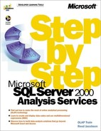
2. | Click the parent-child option, and click Next. Then select the Scenario table, and click the Browse Data button.
| |
3. | Close the Browse Data window, and click Next. | |
4. | Select Scenario_ID as the member key, Parent_ID as the parent key, and Scenario as the member name. Then click Next twice. | |
5. | Type Scenario as the name of the dimension, and click Finish. Click the Data tab, and expand the All Scenario member to browse the dimension. In a Scenario dimension, you do not want an All level. Summing the values of the scenarios is never appropriate. | |
6. | In the Dimension Editor’s dimension tree, select the Scenario dimension, and on the Advanced Tab of the Properties pane, change the All Level property to No. | |
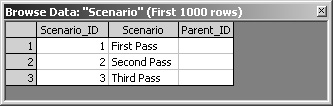
7. | Change the Write-Enabled property to True.
| |
8. | In the dimension tree, select the Scenario Id level, and change the Level Naming Template property to Scenario. | |
9. | Save the dimension, and close the Dimension Editor. |
You now have a shared, single-level, write-enabled, parent-child Scenario dimension that you can use in creating a sales forecast cube.
Create a Cube from an Empty Fact Table
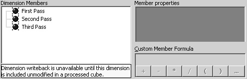
Logically, since all the values in the sales forecast cube will be hand-entered by you, the cube should not require a fact table. As you’ll soon learn in “Enable write-back for a cube,” that’s because when you write values back to a cube, they’re not stored in the fact table. Physically, however, you cannot create a cube without a fact table. If for no other reason, the columns of the fact table determine the potential dimensions and measures for the cube. The Chapter4.mdb sample database includes a fact table named ForecastFact. It has columns for three dimension keys: Category_ID, Quarter_ID, and Scenario_ID. It also has a column for a single measure: Sales_Units. The table is, however, completely empty. It does not, and never will, contain any rows. You must have a fact table to create a cube, but nobody said the fact table had to contain facts.
1. | Right-click the Chapter 4 database Cubes folder, point to New Cube, and click Editor. |
2. | Select ForecastFact as the fact table, and click OK. Click Yes when cautioned about how long it will take to count the fact table rows. Click OK. |
3. | Right-click the heading of the ForecastFact table, and click Browse Data.
|
4. | |
5. | Right-click the Dimensions folder, and click Existing Dimensions. Double-click the Scenario dimension, and click OK. |
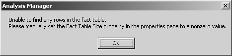
6. | If warned that an automatic join is not possible, click OK and drag the Scenario_ID column from the ForecastFact table onto the Scenario_ID column of the Scenario table. With one measure and one dimension, you should now have all you need to save and process the cube. If you were to try, however, you would see a message informing you that there are no rows in the fact table. Before processing a cube from a fact table with no rows, you must manually enter a nonzero value as the number of fact table rows. In other words, you must lie.
|
7. | In the cube tree, select the cube, and on the Advanced tab of the Properties pane, type 1 as the value of the Fact Table Size property. (Any number greater than 0 will do.) |
8. | Click the Process Cube button, accept the offer to save the cube, decline the offer to design storage, accept the default processing method, and close the Process log window. Click the Data tab to browse the cube.
|
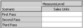
Not surprisingly, the Sales Forecast cube is empty. The important points are that it exists and that it has placeholders where you can add forecast values.
Use Only the Top Levels of a Shared Dimension
You’ll forecast sales by product category and by quarter. Product categories are found in the Product dimension, but they’re not at the lowest level of the dimension. Likewise, calendar quarters are found in the Time.Calendar dimension, but, again, they’re not at the lowest level of the dimension. One possibility would be to create new, private dimensions just for this cube. You don’t want to do that, however, because doing so would prevent you from comparing forecast values from the Sales Forecast cube with actual values from the Sales cube. Rather, you must figure out how to use only part of an existing shared dimension in the new cube.
1. | |
2. | Drag the Category_ID column from the ForecastFact table onto the Category_ID column of the Product Category table. (You might want to rearrange the tables to make them easier to see.) 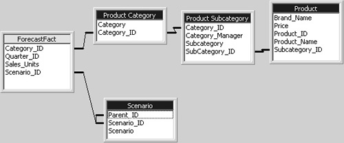
|
3. | Expand the Product dimension, and select the Subcategory level. On the Advanced tab of the Properties pane, change the Disabled property to Yes. Disabling the Subcategory level automatically disables the Product Name level. The Disabled property is a property of a level, but it exists only within the Cube Editor. It wouldn’t make sense to disable a level in the Dimension Editor because that would disable it for all cubes. Disabling a level does not merely hide the level from view; it completely removes that level and all levels below it from the dimension, as far as the current cube is concerned. |
4. | Right-click the Dimensions folder, and click Existing Dimensions. Double-click the Time.Calendar dimension, and click OK. Click OK when warned that no automatic join was found. |
5. | Drag the Quarter_ID column from the ForecastFact table onto the Month_ID column of the TimeMonth table. 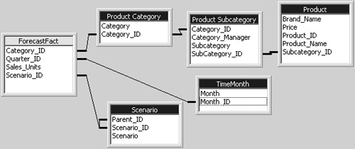 You can join the Quarter_ID of the fact table to the Month_ID of the TimeMonth table because Quarter_ID does refer to a month; it just refers to the first month in the quarter.
 |
6. | |
7. | Click the Process Cube button, accept the offer to save the cube, decline the offer to design storage, select the Full Process processing method, and close the Process log window. Click the Data tab to browse the cube. |
8. | Drag the Product dimension to the Rows axis (exchanging places with Scenario). Drag the Time.Calendar dimension to the Columns axis (exchanging places with Measures). Expand the 1998 member. Scroll the grid until you can see the quarter columns. 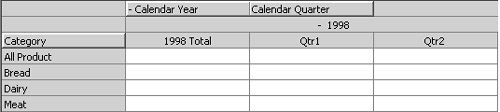
|
9. | Close the Cube Editor. |
Shared dimensions can be, well, shared between multiple cubes. But cubes do not always have the same level of detail. The Disabled property of a dimension level allows you to customize a shared dimension to work with the cube at hand.
Enable Write-back for a Cube
In Analysis Services, you can write values only to the lowest level of a cube. In other words, you cannot change the value of an aggregation. If you could change the value of an aggregation, you would be able to make the cube internally inconsistent. Technically, Analysis Services writes incremental change values either to the client cache in the PivotTable service or to a special write-back table in a relational database. Analysis Services then dynamically combines the write-back values with any values from the fact table.
Note
For application developers, Analysis Services includes a tool—the Update Cube MDX statement—that will allocate a given high-level input value to create the necessary lowest-level values. A client application can thus appear to write back at a high level. In reality, however, the values being written back to the cube are always at the lowest level of the cube.
To write values back to a cube, you must have a client application that includes write-back capabilities. None of the browsers included with Analysis Services or with Microsoft Office 2000 includes write-back capability. Included on the companion CD for this book is a Microsoft Excel 2000 workbook that includes macros that demonstrate how to write values back to the Sales Forecast cube of the Chapter 4 database.
Write Values Back to a Cube Temporarily
When performing a what-if analysis, you might want to write values back to a cube without making them permanent or visible to other users of the cube. Analysis Services allows you to write values back to the PivotTable services cache, which makes them temporary and private.
When a client application allows you to write back to a cube, that means you can write back to any cube, even a local cube. But, unless the cube is write-enabled, the write-back values are only stored within the PivotTable Service cache, which makes them invisible to any other users of the cube and makes them disappear when the current connection to the cube terminates.
|
Local cube files are explained in “Creating a Local Cube” in Chapter 5, “Office 2000 Analysis Components.” |
Write Values Back to a Cube Permanently
To write values back so that others can see them or so that they’ll be retained for future use, the cube must be write-enabled. When you write-enable a cube, you specify the location of a relational table where the write-back values will be stored.
1. | In Analysis Manager, expand the Cubes folder in the Chapter 4 database and right-click the Sales Forecast cube. When the Write-enable dialog box appears, accept the default data source and table name and click OK.
Note You don’t need to write the data back to the same data source as the one containing the fact table. For example, if the fact table for the cube is in a corporate data warehouse that you don’t have permission to write to, you can create a Microsoft Access or Microsoft SQL Server database that you can use for the write-back table. The Write-enable dialog box even allows you to define a new data source dynamically. | |
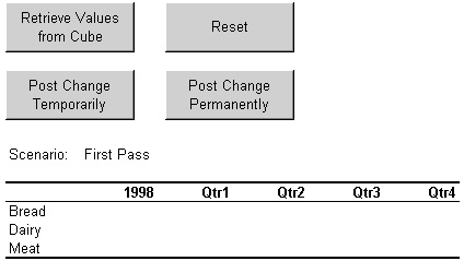
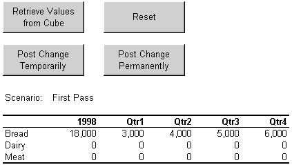
2. | Switch back to the Writeback workbook in Excel, and click Reset so that the PivotTable Service will create a new session that uses the write-back setting for the cube. Then click Retrieve Values From Cube. The original empty cells and labels appear. | |
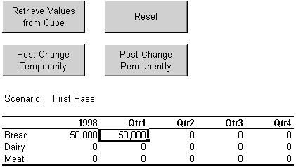
3. | In the Bread row, type 3,000 for Qtr1 (D13), 4,000 for Qtr2 (E13), 5,000 for Qtr3 (F13), and 6,000 for Qtr4 (G13). Then click Post Change Permanently. | |
4. | Click Reset, which clears the data range and resets the connection to the server, and then click Retrieve Values From Cube.
| |
5. | Change the scenario name in the worksheet (cell C10) from First Pass to Second Pass, and click the Retrieve Values From Cube button. | |
6. | In the Bread row, type 3,500 for Qtr1 (D13), 4,500 for Qtr2 (E13), 5,500 for Qtr3 (F13), and 6,500 for Qtr4 (G13). Then click Post Change Permanently. You can write back to a cube in Analysis Services in either of two modes: you can write back only to the PivotTable Service cache, which would be useful for temporary what-if analysis, or you can write back to a relational table, which is useful for sharing changes with other users. To write back to a relational table, you must explicitly write-enable the cube.
Note If you know Microsoft Visual Basic and want to create your own application that can write values to a cube, look at the macros in the Writeback workbook for some useful sample code. | |
7. | In Analysis Manager, right-click the Sales Forecast cube. Point to Write-Back Options, and click Browse Writeback Data. The Browse Data window appears, showing the rows contained in the write-back table. You can resize the window as necessary to see all the columns. 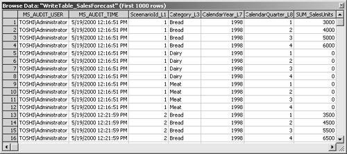 The MS_AUDIT_USER and MS_AUDIT_TIME columns on the left contain audit-trail information: the name of the user who made the changes, and the time the changes were made. The SUM_SalesUnits column on the right contains the measure for the cube. (The table includes one column for each measure in the cube.) The remaining columns contain the member keys for each level of each dimension in the cube.
The write-back table stores incremental values. If you were to change the value of First Pass value for Bread in Qtr1 of 1998 to 4,000 and write the value back to the cube again, you would get an additional row with new audit information and the value 1,000. | |
8. |

Dynamically Add Members to a Dimension
In the course of a planning cycle, it’s often necessary to add one more round than originally planned—preferably without disrupting the use of the data. Because you write-enabled the Scenario dimension, you can easily add a new scenario. Typically, writing new values into a dimension is something that a client application would help you do. Fortunately, the dimension browser in Analysis Manager will allow you to write new values to a dimension.
|
You can also write back to a shared dimension from the Dimension Editor. |
1. | In Analysis Manager, right-click the Sales Forecast cube and click Edit. |
2. | In the Dimensions folder, right-click the Scenario dimension and click Browse. |
3. | |
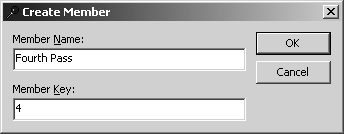
4. | Type Fourth Pass as the name of the new member, and click OK. You can see the new Scenario_ID that will be assigned to the scenario. Unlike writing back values to a cube—where values are stored in a special write-back table—when you add a new member to a dimension, the member is added directly to the original dimension table. You must have permission to add rows to the dimension table in order to use dimension write-back.
|
5. | |
6. | Switch to Excel, and change the name of the Scenario (in cell C10) from Second Pass to Fourth Pass, the newly created Scenario name. Then click the Retrieve Values From Cube button. You don’t need to process the cube or the dimension in order for new dimension members to take effect. The process is remarkably seamless. |
7. | |
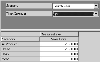
8. | In the Cube Editor, click the Data tab. Select Fourth Pass in the Scenario dimension and Qtr1 of 1998 in the Time Calendar dimension to see the new values in the Bread and All Product cells.
|
9. | Close the Cube Editor. |

The ability to dynamically create new members—particularly for a Scenario dimension—is critical for a planning application. In this section, you’ve seen how the write-back process works, but only with limited tools. If planning will be a part of your work with Analysis Services, you’ll need to obtain or create a client application that supports write-back—at least for cube data.