
Creating an Internet Tracking Cube
Sometimes you might have information in a table that doesn’t look like a standard star schema, with separate fact and dimension tables. For example, suppose that your company has a Web site and maintains a log of people who visit the site. In such a situation, the log file might contain nothing more than a Visitor ID and a date—certainly no discernible measure column. You need to be able to create a cube from a “fact” table that doesn’t have a measure.
Also, the Analysis server has a limitation that there can be no more than approximately 64,000 children for any one parent in a hierarchy. A log of visitors could easily exceed that number of different visitors many times over, with no information available for building a hierarchy.
Create a Cube from a Measureless Fact Table
The Chapter4.mdb sample database contains a Visits table with only two columns: Visitor_ID and Day. Although the table is relatively small, it can give you an idea of how to deal with a large, flat fact table with no apparent measures.

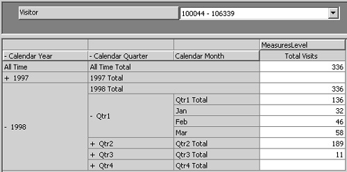
The number 45,225 corresponds to the number of rows in the Visits fact table. For each visitor, you can see the number of times that person visited the site. You cannot, however, see the specific days for the visits.
Enable Drillthrough for a Cube
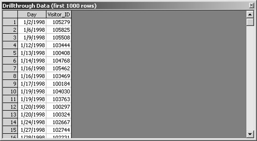
Drillthrough is a feature that allows you to see the individual rows from the fact table that went into a specific value in the cube.
1. | On the Tools menu, click Drillthrough Options. |
2. | In the Cube Drillthrough Options dialog box, select the Enable Drillthrough check box, click the Select All button, and click OK. Click OK when warned that the cube must be saved. 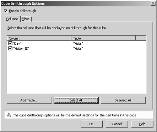
|
3. | |
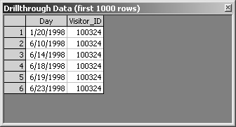
4. | Double-click the Visitor Id cell for Visitor 100324, the one with six visits.
|
5. | Close the Drillthrough Data window. |
Drillthrough is a useful feature, but it might not go as far as you might like. If transaction tables in a database provided the data for the warehouse fact table, you might like to drill through to see the values from the original source tables. Enabling drillthrough for a cube does not provide access to original source data—only to the fact table. Even though drillthrough goes only to the fact table, it can be extremely useful in many situations. And it’s very easy to implement.
Handle a Very Large, Flat Dimension
If the Visits table contained more than 64,000 unique Visitor_ID values, processing the dimension would have failed. That’s because a parent in a hierarchy can have only 64,000 children. If a dimension is large and flat, it can easily exceed 64,000 members—with no suitable information available for grouping the members. A large log of visitors could easily have millions of different members in a dimension. Even though the Visits table has only a few thousand members, you can learn the tools for handling very large, flat dimensions.
|
In “How the Analysis Server Processes a Dimension” in Chapter 9, “Processing Optimization,” you’ll learn why a parent can have only 64,000 children. |
1. | Click the Schema tab to display the Visits table. Drag the Visitor_ID column onto the Visitor level of the Visitor dimension. |
2. | Change the name of the new level to Visitor Group. |
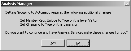
3. | With the Visitor Group level selected, on the Advanced tab of the Properties pane, change the Grouping property to Automatic and press Enter.
|
4. | Click Yes to accept the proposed changes. The new groups are not added to the dimension until you process the cube. |
5. | Click the Process Cube button, accept the offer to save the cube, decline the offer to design storage, accept the default processing method, and close the Process log window. Then click the Data tab to browse the cube. |
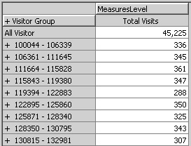
6. | If both the Visitor Group and the Visitor levels are visible, double-click the Visitor Group level heading to collapse it. You can see how the Visitor Group level automatically groups visitors.
|
7. | Expand the first group of visitors. Each group contains individual visitors. Even if the groupings are not meaningful, they help manage an otherwise unwieldy list.
Note You have no direct control over the number of groups created by automatic grouping. Automatic grouping creates approximately the same number of groups as there are members in each group. It does that by using the square root of the number of members. (In the Visits table, there are 17,389 unique visitors. The square root of 17,389 is approximately 132, and there are 132 groups in the Visitor Group level.) This strategy enables grouping to automatically handle dimensions with over 4 billion members (64,000 groups with 64,000 members each). If you want to control the groups, create an expression for the Member Key Column and Member Name Column properties, as explained in Chapter 3. For example, the expression Left(“Visits”.“Visitor_ID”,3) would group the visitors by the first three digits. |

Link Days to a Time dimension
The Visits table contains a Day column. This is a Date/Time column that contains the actual date of the visit. A Date/Time column can be used to support a Date hierarchy. If you create a new, private dimension based on the Day field, you will not be able to compare the values in the Visits cube with those of other cubes in the database, such as the Sales cube. Whenever possible, you should use a shared dimension—particularly for the Time dimension—so that you can compare values between cubes. The Time.Calendar dimension, however, includes only Month, Quarter, and Year levels, while the Visits table contains only daily date values. By using an intermediate table, you can still use the shared dimension in conjunction with daily data.
|
Comparing values between cubes is explained in the section “Combine measures from multiple cubes,” later in this chapter. |
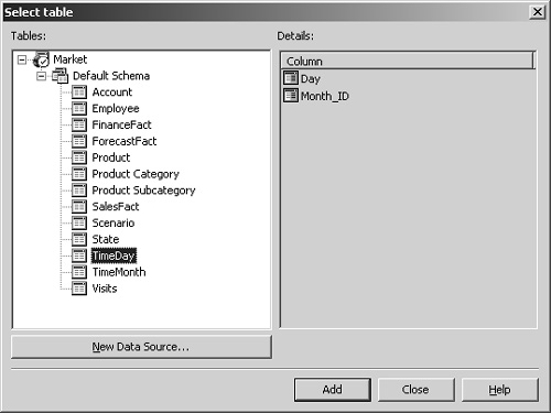 Adding the table should automatically create a join between the Day field of the Visits table and the Day field of the TimeDay table. You must manually create the join between the TimeDay table and the TimeMonth table.
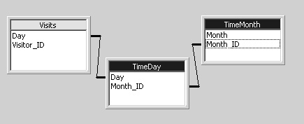
Sometimes you need to create a cube from a fact table that has more detail than a shared dimension you want to use. If you can create an intermediate table that allows the Analysis server to find the relationship between the fact table and the dimension, you can still use the shared dimension. In the section “Use only the top levels of a shared dimension,” later in this chapter, you’ll learn how to use a shared dimension when the fact table is more summarized than the lowest level of a shared dimension.
Calculate Distinct Counts for a Dimension
The Total Visits measure is useful for determining how many visits your site received, but it doesn’t tell you how many different visitors came. Perhaps three people accounted for 90 percent of the visits. To determine how many different visitors came to the site, you need to use the Distinct Count aggregation function. The Distinct Count function is extremely useful, but it has some important restrictions:
Unlike the Count aggregation function, the fact table Source Column for the measure is critical; it determines what you’re counting.
Only one measure in a cube can use the Distinct Count function.
You cannot use Distinct Count for a measure if any dimensions in the cube use custom rollup operators or formulas.
|
See “Understand Analysis server aggregations” in Chapter 8 for performance implications of a measure using a Distinct Count function. |
|
Custom rollup operators are explained in “Use custom rollup operators,” earlier in this chapter. |
Using a Distinct Count aggregation function has restrictions because it’s an extremely powerful analytical tool. Fortunately, the server does the difficult work behind the scenes. Adding a measure that uses Distinct Count to a cube is easy to do:

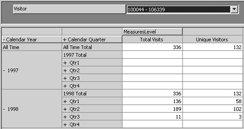
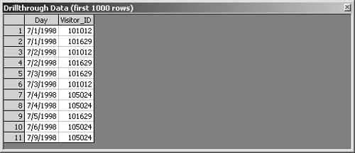
When there are relatively few rows, drilling through to the fact table detail rows can help you see how the same visitor can be responsible for several different visits. The Distinct Count aggregation function highlights those patterns.