
13. Analyzing Data
In This Chapter
• Sorting list information
• Filtering list information
• Transposing row and column information
• Asking “What If?”
• Combining data in a spreadsheet
As you learned in Chapter 12, “Setting Up a Database in Quattro Pro,” a database is a collection of similar information like your local telephone book. In this chapter, you’ll learn how to sort and filter the information in a Quattro Pro database, and then we’ll touch on some of the other analysis tools available in Quattro Pro that are not necessarily related to a spreadsheet database. I’ll show you how to transpose information in rows and columns and then we’ll explore using the What-If Expert to see what happens if you substitute different values into a formula. Then, we’ll combine values in different cells and create an outline in a spreadsheet.
Sorting Data
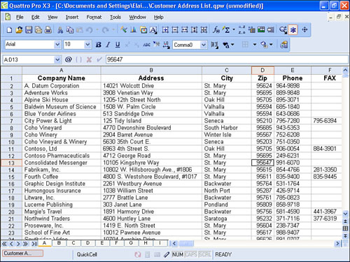
Sorting data in a spreadsheet database is a common activity. Suppose, for example, that your spreadsheet database is a customer mailing list and you want to send out a bulk mailing to all your customers. The post office requires that you sort bulk mailings by Zip Code, so let’s sort the spreadsheet database shown in Figure 13.1 by Zip Code.
Figure 13.1. A customer mailing list currently sorted by name that needs to be sorted by Zip Code.
To sort a spreadsheet, click anywhere in the column by which you want to sort to establish a primary sort key. In this example, I clicked in the Zip column. Then, open the Tools menu and click Sort. Quattro Pro displays the Data Sort window shown in Figure 13.2.
Figure 13.2. Use the Data Sort window to set up the way you want to sort the selected information.
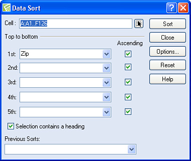
Quattro Pro is smart enough to select the range of cells that makes up the spreadsheet database as the range of cells you want to sort. And, because you placed the cell locator in the column you wanted to sort, Quattro Pro sets up that column heading as the first sort; you can change the first sort to any other column in the spreadsheet by opening the first list and selecting a different column.
Tip

Before you sort, save your spreadsheet. The easiest way to recover from a sort you didn’t expect is to click the Undo button or close the spreadsheet without saving and then reopen it.
As you can see, you can establish up to five sorts for the spreadsheet. Quattro Pro uses the second sort to break ties when it finds multiple occurrences of a value in the first sort field. For example, you might expect to find several customers with addresses in the same Zip Code; you could then establish the company name as the second sort and Quattro Pro will sort the spreadsheet first by Zip Code and, within each Zip Code, by company name.
Tip
You can set sorting options that enable you to sort blank cells first and numbers last. Click the Options button in the Data Sort window.
By default, Quattro Pro sorts information in ascending order; you can sort in descending order by removing the check from the Ascending check box.
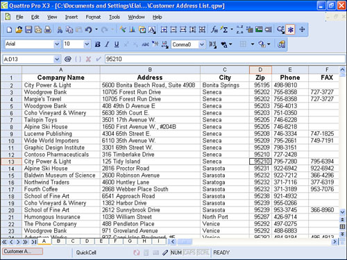
When you click Sort in the Data Sort window, Quattro Pro reorders the selected data based on the criteria you established; in Figure 13.3, the database records now appear in Zip Code order.
Figure 13.3. The database sorted in Zip Code order.
Filtering Information
When you filter information, you hide from view any data that do not meet some criteria you establish. In a spreadsheet database, you can easily filter information by any field in a database record.
Tip
Note that you also can sort the information by any column using the QuickFilter feature.
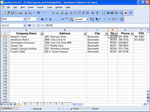
Suppose, for example, that your spreadsheet database is a customer mailing list and you need to send a mailing to customers in a particular town. You can filter the database to display only the customers in that town, and I’ll use the same spreadsheet shown in Figure 13.1 to display only those customers located in Backwater.
First, open the Tools menu and click QuickFilter. Quattro Pro adds a list box down arrow to the first row of the spreadsheet database (see Figure 13.4).
Figure 13.4. When you select the QuickFilter command, Quattro Pro adds a list box down arrow to the first row of your data.
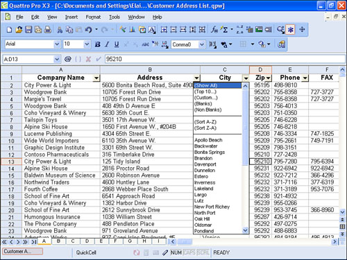
Click any list box down arrow in any column, and Quattro Pro displays the choices by which you can filter. Click any choice in the list and Quattro Pro displays only the records that contain the choice you select; in Figure 13.5, I selected Backwater.
Figure 13.5. The list after hiding all records except those containing the city of Backwater.
To redisplay all records, open the same list box arrow and click Show All.
Transposing Rows and Columns
Transposing rows and columns can come in handy if you discover that your spreadsheet would have worked better if your rows had been columns and your columns had been rows. The Transpose feature lets you switch rows and columns.
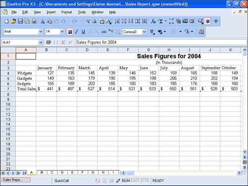
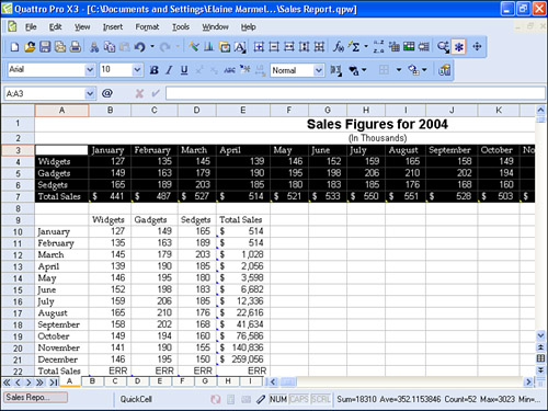
Consider the spreadsheet shown in Figure 13.6; it would probably be easier to read if the months appeared down the side as row headings and the items being sold appeared across the top as column headings—and, of course, the appropriate data would appear in the appropriate cell.
Figure 13.6. A spreadsheet that could benefit if the rows and columns were swapped.
When you switch rows and columns, Quattro Pro copies the information you select to a new area of the spreadsheet, switching rows with columns and columns with rows in the process. Make sure that you have enough blank space in the destination area to accommodate the information; otherwise, Quattro Pro will overwrite the contents of the destination area with the transposed data.
To switch the rows and columns, follow these steps:
- Select the data you want to transpose; for this example, I selected A3.N7.
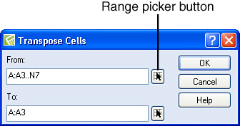
- Open the Tools menu, point to Numeric Tools, and click Transpose. Quattro Pro displays the Transpose Cells dialog box shown in Figure 13.7. The range you want to transpose appears in the From box.
Figure 13.7. Use this dialog box to identify the range containing the data you want to transpose and the range where you want the transposed data to appear.

Quattro Pro does not adjust formulas when you transpose rows and columns. Be sure to edit or reenter formulas as necessary.
- Click the Range Picker button in the To box; Quattro Pro collapses the Transpose Cells dialog box so that you can work in the spreadsheet (see Figure 13.8).
Figure 13.8. Select the upper-left corner of the range where the transposed information should appear.
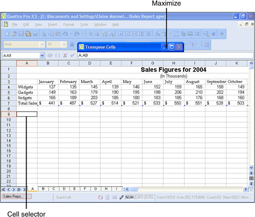
- Click the cell that should become the upper-left corner of the newly transposed range; for this example, I clicked A10.
- Click the Maximize button on the title bar of the Transpose Cells dialog box. The Transpose dialog box reappears, displaying the cell you selected in the To box.
- Click OK. Quattro Pro swaps the information in the rows and columns and displays the information starting in the cell you selected in the To box (see Figure 13.9).
Figure 13.9. The spreadsheet after transposing the rows and columns.
Creating What-If Tables
You can use “What-If” tables in Quattro Pro to see the effects of substituting different values for variables in formulas. Suppose, for example, that you are thinking about buying a house. You’ve determined that the purchase price is $125,000 and you’re going to put down 20% as your down payment and borrow $100,000 for 30 years. Mortgage rates are readily available at 8.5%, but you’d like to know what your monthly mortgage payment would be if you paid points to lower the annual interest rate on the loan. You want to know what your monthly mortgage payment would be for each annual interest rate between 5% and 8.5% in half-point increments. Essentially, your “what-if” question is, “What will my monthly mortgage payment be if the annual interest rate on my loan is 8.5%? 8%? 7.5%? 7%?” and so on.
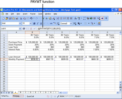
To answer your question, you use the PAYMT function, which requires a monthly interest rate, a loan term, and a loan amount as the three variables it uses to calculate a monthly mortgage payment. You should use the same timeframe for the interest rate and the loan term to accurately calculate the payment. Because you want to calculate a monthly mortgage payment, express the interest rate and the loan duration in months when you set up the formula; divide the annual interest rate by 12 and multiply the number of years on the loan by 12. You can see the sample formula in the Formula bar in Figure 13.10.
Figure 13.10. You can copy and paste your loan assumption information as many times as necessary to calculate monthly mortgage payments at varying interest rates.
You can set up the formula for each of your scenarios, as shown in Figure 13.10, by copying and pasting loan assumption information enough times to test all the interest rates you want. Then, edit each interest rate cell, shown in row 7, to supply a different rate. This method makes you work harder than you need to work, however.
Instead, you can set up a one-variable What-If table, shown in Figure 13.11. In this case, you supply the loan assumptions only once without specifying an annual interest rate. Then, you set up a two-column table to act as your What-If table. The left column of the table contains the values you want to substitute in your calculation; in Figure 13.11, these values appear in B9.B16.
Figure 13.11. The interest variable of the PAYMT function stored in C8 points to B8, the input cell of the two-column What-If table.
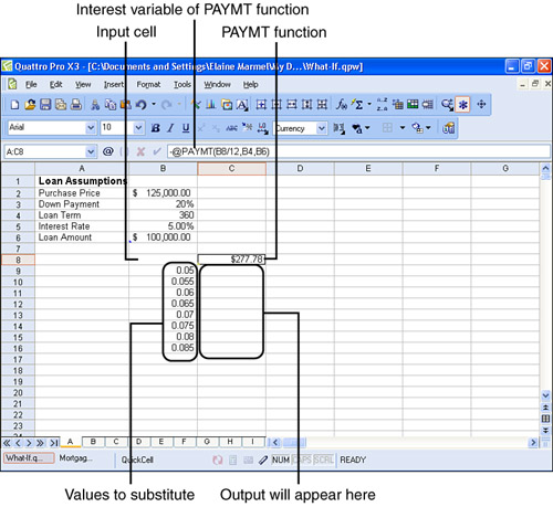
In the PAYMT formula, the first variable is the interest rate. In Figure 13.11, I divided the annual interest rate by 12 to calculate the monthly interest rate of a monthly mortgage payment.
In the right column of the table and in the cell above the first value you want to test, type the formula you want Quattro Pro to use when it substitutes values—in this case, the PAYMT function shown in cell C8. Make sure that one variable of the formula points to the blank cell in the top-left corner of the table—the cell immediately above the values you want to test and to the left of the formula. This blank cell is called the input value, and in this example, I used B8 as the input cell for the variable in the PAYMT formula that I want to test.
Then, open the Tools menu, point to Numeric Tools, and click What-If Tables. Quattro Pro displays the What-If window shown in Figure 13.12.
Figure 13.12. Use this window to identify the What-If table components.
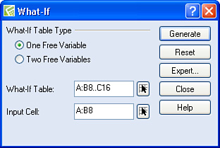
A one-variable What-If table enables you to substitute a value for one variable in a formula. Quattro Pro can calculate one-variable and two-variable What-If tables.
Select the One Free Variable Option and then click the Range Picker button beside the What-If Table option. When Quattro Pro collapses the window, select the cells containing both the formula you want to calculate and values you want to substitute in the formula; in this example, I selected B8.C16.
Next, click the Range Picker button beside Input Cell option and select the blank cell above the substitution values and to the left of the formula; in this example, I selected B8.
Click the Generate button, and Quattro Pro places, in the cells beside the various interest rates, the result of the formula obtained by changing the variable in the formula that points to the input cell at the upper-left corner of the What-If table (see Figure 13.13).
Figure 13.13. A one-variable What-If table that calculates monthly mortgage payments for annual interest rates between 5% and 8.5%.

Consolidating Data
You can consolidate data from different locations in the same notebook or even from different notebooks. When you consolidate data, Quattro Pro combines the information in cells you specify to provide the results.
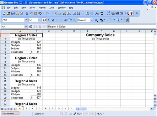
Suppose, for example, that you have collected and entered sales information for three products across three regions. Now, you need the total sales for each product across all regions. Your data might look something like Figure 13.14, in which I’ve set up an area in the spreadsheet where I’d like the consolidated information to appear. Although I’m going to show you how to add like values in each set of data, Quattro Pro can also combine the values and average, count, and calculate the minimum or maximum values, the standard deviation, the variance, the sample standard deviation, or the sample variance of the data.
Figure 13.14. A spreadsheet containing individual product sales for four regions that needs to be consolidated into a company total.
To successfully consolidate data, your data should have common row or column labels in each set of data you want to consolidate. The values in each set of data do not need to appear in the same order nor do you need to have the same number of values in each data set. In my example, I used three products in each region to make it easy for you to see how consolidation works, but I could just as easily have had two products in one region, three products in two regions, and four products in another region. Quattro Pro combines the values of cells with common labels.
To consolidate the data, follow these steps:
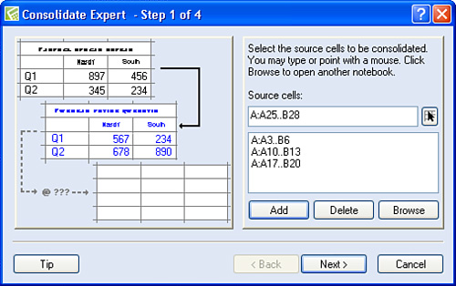
- Open the Tools menu, point to Consolidate, and click New. Quattro Pro displays the first step of the Consolidate Expert.
- Click the Range Picker in the Source Cells box to collapse the Consolidate Expert and identify the first set of data to consolidate. In this example, I selected A3.B6.
- Click the Maximize button in the collapsed window to redisplay the Consolidate Expert and click the Add button. Quattro Pro adds the range in the box below the Source cells box.
- Repeat steps 2 and 3 for each range you want to consolidate. In Figure 13.15, I am just about to add the fourth region’s sales data to the consolidation.
Figure 13.15. Define the regions to consolidate.
- Click Next. step 2 of 4 of the Consolidate Expert appears (see Figure 13.16).
Figure 13.16. Select an operation for the consolidation.
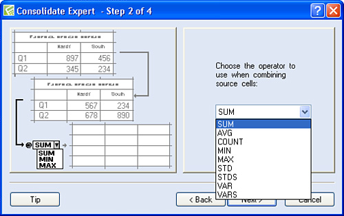
- Click the list box arrow to select the operation you want Quattro Pro to perform when it consolidates the data.
- Click Next. step 3 of 4 of the Consolidate Expert appears (see Figure 13.17).
Figure 13.17. Identify the destination for the consolidated cells.
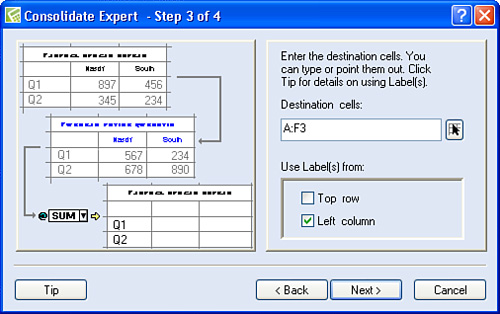
- Click the in the Destination Cells box to collapse the Consolidate Expert and identify the destination for the consolidated data. You can identify a single cell, and Quattro Pro will use surrounding cells as needed for the consolidated data. In this example, I selected F3.
Caution

Quattro Pro will overwrite any data in the destination range with the consolidation information, so be sure to select an empty area of the spreadsheet.
- Click Next. step 4 of 4 of the Consolidate Expert appears (see Figure 13.18).
Figure 13.18. Assign a name to the consolidation.
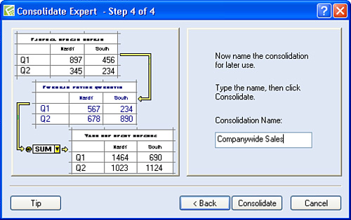
- Type a name for the consolidation in the Consolidation Name box.
- Click Consolidate. Quattro Pro performs the consolidation and places the results in the destination cell range (see Figure 13.19).
Figure 13.19. Consolidated data appears in F3.G6.
Tip
If the source cell range includes labels, you can assign those labels to the destination cell range by selecting the Top Row check box, the Left Column check box, or both. Quattro Pro will organize the data in the destination range using the order of the first source cell range.
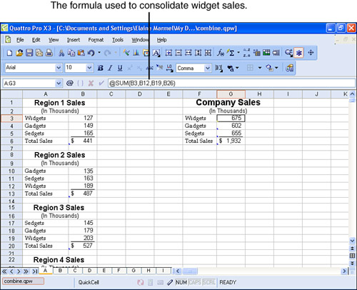
In Figure 13.19, I highlighted G3 so that you can see its contents in the Formula bar; notice that Quattro Pro used the @SUM function to add the values for widgets in each of the three regions and present their consolidated total.
Tip
You can change consolidation settings by opening the Tools menu, pointing to Consolidate, and clicking Edit. Then, select the consolidation you named and change settings.