CHAPTER 24. Overview of the TCP/IP Protocol Suite

SOME OF THE MAIN TOPICS IN THIS CHAPTER ARE

---

TCP/IP and the OSI Reference Model 360

The Internet Protocol (IP) 364

The Address Resolution Protocol—Resolving IP Addresses to Hardware Addresses 380

The Transmission Control Protocol (TCP) 386

The User Datagram Protocol (UDP) 395

Ports, Services, and Applications 397

The Internet Control Message Protocol (ICMP) 398

TCP/IP is the primary network protocol used on the Internet. Unlike many earlier network protocols—such as ARCnet and DECnet—TCP/IP was not developed by a single vendor as a proprietary solution. TCP/IP was created to provide a network link between computer hardware and software platforms from various vendors (such as IBM and Digital Equipment Corporation at the high end, as well as personal computers at the low end). By standardizing on a single set of protocols, each of which serves a specific function, TCP/IP can be used to create a network, no matter what underlying hardware is used. During the early years of TCP/IP, universities, businesses, and government organizations were able to exchange information on the ARPANET—the Internet’s predecessor—because TCP/IP could be implemented on just about any kind of computer. It is easy to implement TCP/IP on a wide variety of operating systems because TCP/IP was developed with a layered approach, which means that network functionality was compartmentalized into layers instead of the traditional approach of writing network drivers as single programs tied to specific hardware.

Using this layered approach means that a vendor need only write a low-level driver for their hardware to work with the upper layers of the TCP/IP code (which provides a standard interface). By freeing the development of the protocol(s) from the hands of particular manufacturers, TCP/IP has been developed to satisfy the needs of the many, instead of the needs of a single vendor’s proprietary hardware. TCP/IP has evolved over time, using a process in which many individuals have had the opportunity to supply input into its development. The Request for Comments (RFCs) documents that you hear about all through this book are the documents that allow suggestions for protocol enhancements and new protocols to be reviewed by a diverse group of individuals who specialize in the particular topic at hand. Although many projects created by a committee turn out to be unwieldy, cumbersome works, this is not the case with TCP/IP. Instead, the RFC process allows for a great deal of input when creating standards, often resulting in a higher quality standard after scrutiny by experts in the field.

In this chapter, we will look at all the major protocols that make up the TCP/IP suite and show how they work together. In addition to the protocols you will read about here, the TCP/IP suite includes some standard applications, such as FTP and Telnet. These are discussed in Chapter 25, “Basic TCP/IP Services and Applications.” Finally, in Chapter 27, “Troubleshooting Tools for TCP/IP Networks,” you will find useful information about programs that were written to help diagnose problems when this complex suite of protocols and applications doesn’t appear to be working as it should.

To begin, it is important to understand the basic protocols on which the entire TCP/IP suite is built.

TCP/IP and the OSI Reference Model

As discussed earlier, TCP/IP was built using a layered approach. You may have heard about the OSI (Open Systems Interconnect or Open Systems Interconnection) Reference model that is used mostly as a framework around which a discussion of network protocols can be discussed. Developed in 1984 by the International Organization for Standardization (ISO), this model defines a protocol stack in a modular fashion, specifying what functions are performed by each module.

For further discussion of the OSI reference model, see Appendix A, “Overview of the OSI Seven-Layer Networking Reference Model.”

For the purposes of this chapter, it should be noted that development of TCP/IP began long before the OSI model, and, as can be expected, TCP/IP protocols don’t always neatly match up to the seven layers of the OSI model.

The ISO used this model to develop a set of open network protocols, but these were never widely adopted. This was due to several factors. First, at that time many computer vendors held market share by keeping customers locked into proprietary hardware/software solutions. Second, the OSI protocols required a considerable amount of system resources, so it was impractical to try to implement them on smaller computers, such as minicomputers, much less the now-standard PC. However, the OSI networking model is still used today when discussing network protocols, and it is a good idea to become familiar with it if you will be working in this field. TCP/IP was developed based on a similar, though less modular, reference model, the DOD (Department of Defense) or DARPA model.

In Figure 24.1, you can see the four layers that make up the TCP/IP-DOD model, and how each layer relates to the OSI model.

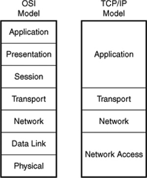
Figure 24.1. Comparison of the TCP/IP and OSI networking models.

As you can see, TCP/IP doesn’t exactly fit into the OSI model, but it is still possible to refer to the model when discussing certain aspects of the protocols and services that TCP/IP provides.

TCP/IP Is a Collection of Protocols, Services, and Applications

The acronym TCP/IP stands for Transmission Control Protocol/Internet Protocol. In addition to these two important protocols, many other related protocols and utilities are commonly grouped together and called the TCP/IP protocol suite. This “suite” of protocols includes such things as the User Datagram Protocol (UDP) and the Internet Control Message Protocol (ICMP), and others discussed in this chapter and in several other chapters in this book.

TCP/IP, IP, and UDP

The main workhorses of this protocol suite are IP, TCP, and UDP:

IP—The Internet Protocol is an unreliable, connectionless protocol that provides the means to get a datagram from one computer or device to another and for internetwork addressing.

TCP—The Transmission Control Protocol uses IP but provides a higher-level functionality that checks to be sure that the packets that IP manages actually get to and from their intended destinations. TCP is a reliable, connection-oriented protocol, requiring that a session be established to manage communications between two points in the network so that errors can be detected and, if possible, corrected.

UDP—The User Datagram Protocol also uses IP to move data through a network. Whereas TCP uses an acknowledgment mechanism to ensure reliable delivery, UDP does not. UDP is intended for use in applications that don’t necessarily need the guaranteed delivery service provided by TCP. The Domain Name System (DNS) service is an example of an application that uses UDP. Applications that make use of UDP are responsible for taking on the functions of checking for reliable delivery that is provided by TCP.

As you can see in Figure 24.2, IP is the basic protocol used in the TCP/IP suite to get datagrams delivered.

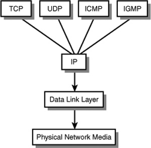
Figure 24.2. IP is used by many other protocols as the mechanism by which their data is routed and delivered through the network.

This figure shows that TCP/IP and its related protocols work above the physical components of the network. Therefore, it is easy to adapt TCP/IP to different types of networks, such as Ethernet and Token-Ring. When you talk about using TCP/IP on the network, what it all boils down to is that you’re packaging your data into an IP packet that is passed down to the actual network hardware for delivery. Because IP is the common denominator of the TCP/IP suite, this chapter covers it first, and after that shows how the remaining protocols build on the functions provided by IP.

Other Miscellaneous Protocols

In addition to TCP and IP, many other protocols are part of the TCP/IP suite. Back in Figure 24.2 you can see that the IGMP and ICMP protocols are included. IGMP is the Internet Group Management Protocol, which is used to manage groups of systems that are members of multicast groups. Multicasting is a technique that allows a datagram to be delivered to more than one destination. Figure 24.2 also shows the Internet Control Message Protocol (ICMP), which performs many functions to help control traffic on a network. In addition to these protocols, which are discussed later in this chapter, other protocols usually considered as part of or associated with the TCP/IP protocol suite include the following:

ARP—The Address Resolution Protocol. ARP is used by a computer to determine what hardware address is associated with an IP address. This is necessary because IP addresses are used to route data between networks, while communications on the local network segment are done using the burned-in hardware address of the network cards.

RARP—The Reverse Address Resolution Protocol is similar to ARP but works in reverse. This is an older protocol that was developed to allow a computer to find out what IP address it should use, based on a table stored on a device such as a router. This functionality has generally been replaced by other protocols, such as BOOTP and DHCP. However, you can still find this protocol in use on many networks that contain older legacy equipment that has yet to reach the end of its useful life, such as diskless X-Windows terminals.

DNS—The Domain Name System is the hierarchical naming system used by the Internet and most TCP/IP networks. For example, when you type http://www.quepublishing.com into a browser, your TCP/IP stack sends a request to a DNS server to find out the IP address associated with that name. From then on, the browser can use the IP address to send requests to the Web site. More information about DNS can be found in Chapter 29, “Network Name Resolution.”

BOOTP—The Bootstrap Protocol is also an older protocol that has generally been replaced by DHCP. In fact, most DHCP servers can act as BOOTP servers as well. BOOTP was created to allow a diskless workstation to download configuration information, such as an IP address and the name of a server that can be used to download an operating system. Because the diskless workstation has no local storage (other than memory), it can’t store this information itself between boots.

DHCP—The Dynamic Host Configuration Protocol relieves the network administrator of the task of having to manually configure each computer on the network with static addressing and other information. Chapter 28, “BOOTP and Dynamic Host Configuration Protocol (DHCP),” covers this topic in great detail.

SNMP—The Simple Network Management Protocol was developed to make managing network devices and computers from a central location easier. You can find out more about SNMP in Chapter 49, “Network Testing and Analysis Tools.”

RMON—The Remote Monitoring protocol was developed to further enhance the administrator’s ability to manage computers and network devices remotely. This protocol is also covered in greater detail in Chapter 49.

SMTP—The Simple Mail Transfer Protocol is the protocol that gets your email from here to there. Chapter 26, “Internet Mail Protocols: POP3, SMTP, and IMAP,” can give you more information about how this protocol functions, along with other email protocols.

The Internet Protocol (IP)

Although the Internet protocol is the second component of the TCP/IP acronym, it is perhaps the more important of the two. IP is the basic protocol in the suite that provides the information used for getting packets from one place to another. IP provides a connectionless, unacknowledged network service, and also provides the addressing mechanism used by TCP/IP. The following main features distinguish IP from other protocols:

IP is a connectionless protocol. No setup is required for IP to send a packet of information to another computer. Each IP packet is a complete entity and, as far as the network is concerned, has no relation with any other IP packet that traverses the network.

IP is an unacknowledged protocol. IP doesn’t check to see that a datagram or packet actually arrives intact at its destination. However, the Internet Control Message Protocol does assist IP so that some conditions can be corrected. For example, although IP doesn’t receive an acknowledgment from the destination of an IP packet, it will receive ICMP messages telling it to slow down if it is sending packets faster than the destination can process them.

IP is unreliable. This is easy to see based on the first two items in this list. IP lacks a mechanism for determining whether packets are delivered, and thus packets can be dropped by routers or other network devices. This can happen, for example, when the network traffic exceeds the bandwidth that a network device can handle.

IP provides the address space for TCP/IP. This is perhaps the most important feature of the IP protocol. The hierarchical nature of IP addressing is what makes it possible to connect millions of computers on the Internet without requiring each computer to know all the addresses on the network.

IP Is a Connectionless Transport Protocol

IP is connectionless—each packet is separate from the others. From the IP standpoint, each packet is unrelated to any other packet. IP does not contact the destination computer or network device and set up a route that will be used to send a stream of data. Instead, it just accepts data from a higher-level protocol, such as TCP or UDP, formats a package that contains addressing information, and sends the packet on its way using the underlying physical network architecture. The information found in the IP datagram header is used on a hop-by-hop basis to route the datagram to its destination. When a higher-level protocol uses IP to deliver a series of information packets, there is no guarantee that each packet created by the IP layer will take the same route to get to the eventual destination. It is quite possible for a series of packets created by a higher-level protocol to reach the destination in a sequence out of order from how they were transmitted. IP doesn’t even care whether packets arrive at their destination. That function is left to the protocol that uses IP for delivery. This doesn’t mean that IP is a useless protocol, however—it just means that the higher-level protocols (such as TCP) that use IP need to provide for some kind of error checking, packet sequencing, and acknowledgment. You’ll learn more about this subject in the section “The Transmission Control Protocol (TCP),” later in the chapter, when we talk about how TCP sets up a connection and acknowledges sent and received packets.

IP Is an Unacknowledged Protocol

IP does not check to see whether the datagrams it sends out ever make it to their destination. It just formats the information into a packet and sends it out on the wire. Thus, it is considered to be an unacknowledged protocol. The overhead involved in acknowledging receipt of a datagram can be significant. Leaving out an acknowledgment mechanism enables IP to be used by other protocols and applications that do not require this functionality, and thus eliminates the overhead associated with acknowledgments. Applications and protocols that do need to know that a datagram has been successfully delivered will not use the IP protocol. Instead, they can implement the acknowledgment mechanism found in the TCP protocol.

One way of thinking about this relationship between IP and upper-level protocols is to consider how the postal service works. If you send a letter through the mail, you have no way to know when—or even whether—the letter was correctly delivered. Unless you pay the extra money to get a signed receipt of delivery returned to you, you can’t be sure that the letter ever reached its destination.

IP Is an Unreliable Protocol

Because IP is connectionless and because it does not check to see whether packets arrive at their destination, and because packets may arrive out of order, IP is considered an unreliable protocol. Or, to put it another way, it’s a best-effort delivery service. IP doesn’t perform routing functions (that task is left up to routers and routing protocols), and IP can’t guarantee what route a datagram will take through the network. Another reason it is considered unreliable is that IP implements a Time to Live (TTL) value that limits the number of network routers or host computers through which a datagram can travel. When this limit is reached, the datagram is simply discarded. Because no acknowledgment mechanism is built into IP, it is unaware of this kind of situation. The reason for this is to solve problems associated with routing. For example, it’s quite possible for an administrator to configure a router incorrectly, causing an endless loop to be created in a network. If it were not for the TTL value, the packet could continue to pass from one router to another, and another, forever. The TTL value is used mainly to prevent just this type of situation from occurring.

IP Provides the Address Space for the Network

Addressing is one of the most important functions implemented in the IP layer. In earlier chapters you learned that network adapter cards use a burned-in address, usually called a Media Access Control (MAC) address. These addresses are determined by the manufacturer of the network card, and the address space created is considered to be a “flat” address space. That is, there is no organization provided by MAC addresses that can be used to efficiently route datagrams from one system or network to another. On an Ethernet card, for example, a MAC address is composed of two parts. The first part of the MAC address identifies the manufacturer of the network card. The remaining octets (or bytes) are assigned, usually in a serial fashion, to the cards the manufacturer produces. The MAC address assigned to each adapter is unique and is made up of a 6-byte address (48 bits), which is usually expressed in hexadecimal notation to make it easier to write. For example, 00-80-C8-EA-AA-7E is much easier to write than trying to express the same address in binary, which would be a string of zeros and ones 48 bits long (in this example, 000000001000000011001000111010101010101001110011).

IP addresses are also made up of two components: a network address and a host address. By allowing a network address, it is possible to create a hierarchy that allows for an efficient routing mechanism when sending data to other networks. Whereas a particular network might consist of systems that have network adapters from multiple vendors, and thus have MAC addresses that are seemingly random numbers, IP addresses are organized into networks. Because of this, routers don’t have to keep hundreds of millions of MAC addresses in a memory cache to deliver datagrams. Instead, they just need a table of addresses that tells them how to best route a datagram to the network on which the host system resides.

Just What Does IP Do?

IP takes the data from the Host-to-Host layer (as shown previously in Figure 24.1) and fragments the data into smaller packets (or datagrams) that can be transferred through the network. On the receiving end, IP then reassembles these packets and passes them up the protocol stack to the higher-level protocol that is using IP. To get each packet delivered, IP places the source and destination IP addresses into the packet headers. IP also performs a checksum calculation on the header information to ensure its validity. Note, however, that IP does not perform this function on the data portion of the packet.

As already noted, TCP/IP allows for networks made up of different underlying technologies to interoperate. While one network might use the Ethernet 802 frame format, another might use FDDI. Each of these lower-level frames has its own particular header that contains information needed by that technology to send frames through the physical network media. At this lower level in the protocol stack, the IP packet rides in the data portion of the frame. After IP adds its header information to the message it receives from a higher-level protocol, and creates a packet of the appropriate size, it passes the packet to the Network Access layer, which wraps the IP packet into an Ethernet frame, for example. At the receiving end the Ethernet frame header information is stripped off, and the IP datagram is passed up the stack to be handled by the IP protocol. Similarly, the IP header information is stripped off by the higher-level protocols that use IP, such as TCP or UDP.

Examining IP Datagram Header Information

In Figure 24.3 you can see the format of an IP packet. In the IP header you will find the addressing information that is used by routers and other network devices to deliver the packet to its eventual destination.

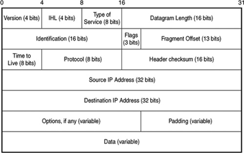
Figure 24.3. The IP header contains information concerning addressing and routing the packet.

These are the header fields of the IP packet:

Version—IP comes in different versions. This 4-bit field is used to store the version of the packet. Currently, IP version 4 is the most widely used version of IP. The “next generation” IP is called IPv6, which stands for version 6. Because different versions of IP use different formats for header information, if the IP layer on the receiving end is a lower version than that found in this field, it will reject the packet. Because most versions of IP at this time are version 4, this is a rare event. Don’t worry about this field until you upgrade your network to IPv6.

Internet Header Length (IHL)—This 4-bit field contains the length of the header for the packet and can be used by the IP layer to calculate where in the packet the data actually starts. The numerical value found in this field is the number of 32-bit words in the header, not the number of bits or bytes in the header.

Type of Service (TOS)—This 8-bit field is intended to implement a prioritization of IP packets. Until recently, however, no major implementation of IP version 4 has used the bits in this field, so these bits are usually set to zeros. With Gigabit Ethernet and 10 Gigabit Ethernet, this is changing. Because these faster versions of Ethernet can compete with other protocols such as ATM, which do provide a type of service function, you can expect to see this field used in faster versions of Ethernet. IPv6 also provides mechanisms that allow this functionality.

Datagram Length—This field is 16 bits long and is used to specify the length of the entire packet. It contains the number of 8-bit octets (or bytes). The largest value that can be stored in 16 bits is 65,535 bytes. Subtracting the IHL field from this value, IP will yield the length of the data portion of the packet.

Identification—IP often must break a message it receives from a higher-level protocol into smaller packets, depending on the maximum size of the frame supported by the underlying network technology. On the receiving end, these packets need to be reassembled. The sending computer places a unique number for each message fragment into this field, and each packet for a particular message will have the same value in this 16-bit field. Thus, the receiving computer can take all the parts and re-create the original message.

Flags—This field contains several flag bits. Bit 0 is reserved and should always have a value of zero. Bit 1 is the Don’t Fragment (DF) field (0 = fragmentation is allowed, 1 = fragmentation is not allowed). If a computer finds that it needs to fragment a packet to send it through the next hop in the physical network, and this DF field is set to 1, then it will discard the packet (remember that IP is an unreliable protocol). If this field is set to 0, it will divide the packet into multiple packets so that they can be sent onward in their journey. Bit 2 is the More Fragments (MF) flag and is used to indicate the fragmentation status of the packet. If this bit is set to 1, there are more fragments to come. The last fragment of the original message that was fragmented will have a value of zero in this field. These two fields (Identification and Flags), along with the next field, control the fragmentation process.

Fragment Offset—When the MF flag is set to 1 (the message was fragmented), this field is used to indicate the position of this fragment in the original message so that it can be reassembled correctly. This field is 13 bits in length and expresses the offset value of this fragment in units of 8 bytes.

Time to Live (TTL)—Were it not for TTL, a packet could travel forever on the network because it is possible for loops to exist in the routing structure (due to an administrator’s error, or the failure of a routing protocol to update routing tables in a timely manner). The TTL value is used to prevent these endless loops. Each time a packet passes through a router, the value in this field is decremented by at least one. The value is supposed to represent seconds, and in some cases in which a router is processing packets slowly, this field can be decremented by more than one. It all depends on the vendor’s implementation. When the value of the TTL field reaches zero, the packet is discarded. Because IP is a best-effort, unreliable protocol, the higher-level protocol that is using IP must detect that the packet did not reach its destination and resend the packet.

Protocol—This field is 8 bits long and is used to specify a number that represents the network protocol for the data contained in this packet. The Internet Corporation for Assigned Names and Numbers (ICANN) decides the numbers used in this field to identify specific protocols. For example, a value of 6 is used to specify the TCP protocol.

Header Checksum—This 16-bit field contains a computed value used to ensure the integrity of the header information of the packet. When information in the header is changed, this value is recalculated. Because the TTL value is decremented by each system that a packet passes through, this value is recalculated at each hop as the packet travels through the network.

Source IP Address—The IP address of the source of the packet. This is a 32-bit-long field. The format of IP addresses is discussed in greater detail later in this chapter.

Destination IP Address—The IP address of the destination of the packet. This also is a 32-bitlong field.

Options—This is an optional variable-length field that can contain a list of options. The option classes include control, reserved, debugging, and measurement. Source routing can be implemented using this field and is of particular importance when configuring a firewall. Table 24.1 lists the option classes and option numbers that can be found in this field.

Padding—This field is used to pad the header so that it ends on a 32-bit boundary. The padding consists of zeros. Different machines and different operating systems work based on different sizes for bytes, words, quadwords (all of which are multiples of 8), and so on. Padding makes it easier to handle a known quantity of data (that is, to pad the header to a known length) than for the system to have to find some other method for determining where a data structure ends. For example, a router must operate quickly. It must perform calculations, look up information in the routing table, and so on. Extracting the header information from a packet can be implemented in hardware or software to make the router work faster by using known quantities of bits.

Table 24.1. Option Classes and Option Numbers

The Options Field and Source Routing

The Options field is optional. Source routing (which is discussed in Chapter 45, “Firewalls”), for example, can be implemented using this field. Although IP usually lets other protocols make routing decisions (that is, the path the packet takes through the network), in most cases it is possible to specify a list of devices for the route instead. As shown in Table 24.1, IP can use two options for routing purposes. These are loose source routing (option number 3) and strict source routing (option number 9).

Hackers can use source routing to force a packet to return to their computer, using a predefined route. Using source routing with TCP/IP should be discouraged. For more information, see Chapter 45.

Each of these techniques for source routing provides a list of addresses that the packet must pass through. Loose source routing uses this list but doesn’t necessarily use it in all cases—other routes can be used to get to each machine addressed in the list. When strict source routing is used, however, the list must be followed exactly; if it cannot, the packet will be discarded.

IP Addressing

Although most people think of IP as the transport protocol used by higher-level protocols, one of its more important functions is to provide the address space used by the TCP/IP suite. Earlier in this chapter we discussed the difficulty of having to create a routing table that consists of hundreds of millions of actual hardware addresses, providing for no built-in organization capability.

IP addresses are used for just this purpose: to provide a hierarchical address space for networks. Each network adapter has a hard-coded network address that is 48 bits long. When data packets are sent out on the wire of the local area network (LAN) segment, this MAC address is used for the source and destination addresses that are embedded in the Ethernet frame, which encapsulates the actual IP packet. After an IP packet reaches the destination network, the router sends the packet out onto the network segment that contains the destination. The MAC address is used from there on to deliver the data. On a LAN segment, MAC addresses can be used efficiently because most LAN segments consist of just a few hundred or a few thousand host computers. This number of addresses can easily be stored in network devices, such as bridges or switches.

IP Addresses Make Routing Possible

Because the IP address is composed of two components, the network address and the host computer address, it is a simple matter to construct routers that use the network portion of the address to route packets to their destination networks. After the packet has arrived at a router on the destination network, the host portion of the address is used to locate the destination computer. Without the capability to designate a network address, as well as a host address, the hierarchical address space could not exist, and routing would require routing tables that literally would have to store every address of every computer or device on the network. In such a scenario the IP address would have no advantage over the MAC address. As it stands, IP gets a packet to the destination network by limiting routing tables to storing only network addresses allowing routing to be a simple and more efficient process.

IP addresses allow you to organize a collection of networks in a logical hierarchical fashion. There are three kinds of IP addresses:

Unicast—This kind of address is the most common type of IP address. It uniquely identifies a single host on the network.

Broadcast—Not to be confused with an Ethernet frame broadcast, IP also provides this capability by setting aside a set of addresses that can be used for broadcasting to send data to every host system on a particular network.

Multicast—Similar to broadcast addresses, multicasting addresses send data to multiple destinations. The difference between a multicast address and a broadcast address is that a multicast address can send data to multiple networks to be received by hosts that are configured to receive the data instead of every host on the network.

Anycast—When Ipv6 nodes need to transmit, each individual node can transmit data to a list (or group) of addresses. This type of transmission is called Anycast and it’s fully supported in IPv6.

Additionally, there are address classes, which are used mainly to define the size of the network and host portions of the IP address.

IP Address Classes

The Internet is a collection of networks that are all joined together by routers to create a larger network. The name itself says it all. The Internet Protocol (IP) makes this possible because it allows for addressing each network that is attached to the Internet, as well as identifying the host computers that reside on each network. When packets are routed through the Internet (or through a private corporate network that uses TCP/IP—an intranet), the IP address is used to get the data to the destination network. When the data packet is delivered to a router on the destination network, the actual hardware address (MAC address) of the computer is used to deliver the packet to the correct computer. This is done by taking the host portion of the IP address and consulting a table that maps hardware addresses to IP host addresses for the local network. If no match is found, the Address Resolution Protocol (ARP) is used on the local wire to find out the hardware address, and it is added to the table.

The important factor here is that it’s possible to assign an address both to networks and to the individual hosts.

An IP address is 4 bytes long (32 bits). Whereas MAC addresses usually are expressed in hexadecimal notation, IP addresses usually are written using dotted-decimal notation. Each byte of the entire address is converted to its decimal representation, and then the 4 bytes of the address are separated by periods to make it easier to remember. As you can see in Table 24.2, the decimal values are much easier to remember than their binary equivalents.

Table 24.2. IP Addresses Are Expressed in Decimal Notation

As you can see, it is much easier to write the address in dotted-decimal notation (150.204.200.27) than to use the binary equivalent (10010110110011001100100000011011).

Because IP addresses are used to route a packet through a collection of separate networks, it is important to know what part of the IP address is used as the network address and what part is used for the host computer’s address.

IP addresses are divided into three major classes (A, B, and C) and two less familiar ones (D and E). Each class uses a different portion of the IP address bits to identify the network. There is a need for classifying networks because there is a need to be able to create networks of different sizes. Whereas a small LAN might have only a few computers or a few hundred, larger networks can have thousands or more networked computers. The class system of IP addresses is accomplished by using a different number of bits of the total address to identify the network and host portions of the IP address. Additionally, the first few bits of the binary address are used to indicate which class an IP address belongs to.

The total number of bits available for addressing is always the same: 32 bits. Because the number of bits used to identify the network varies from one class to another, it should be obvious that the number of bits remaining to use for the host computer part of the address will vary from one class to another also. This means that some classes will have the capability to identify more networks than others. Conversely, some will have the capability to identify more computers on each network.

The first 4 bits of the address tell you what class an address is a member of. In Table 24.3, you can see the IP address classes along with the bit values for the first 4 bits. The bit positions that are marked with an “x” in this table indicate that this value makes no difference in the determination of IP address class.

Table 24.3. The First 4 Bits of the IP Address Determine the Class of the Address

Class A Addresses

As shown in Table 24.3, any IP address that has a zero in the first bit position is a Class A address. The values for the remaining bits make no difference. Also, you can see that any address that has 10 for the first 2 bits of the address is a Class B address, and so on. Remember that these are bit values, and as such are expressed in binary. These are not the decimal values of the IP address when it is expressed in dotted-decimal notation.

Class A addresses range from all zeros (binary) to a binary value of 0 in the first position followed by seven 1 bits. Converting each byte of the address into decimal shows that Class A addresses range from 0.0.0.0 to 127.255.255.255, when expressed in the standard dotted-decimal notation.

Keeping in mind that the class system for IP addresses uses a different number of bits for the network portion of the address, the Class A range of networks is the smallest. That is because Class A addresses use only the first byte of the address to identify the network. The rest of the address bits are used to identify a computer on a Class A network. Because the first bit of the first byte of the address is always zero, this leaves only 7 bits that can be used to create a network address. Because only 7 bits are available, there can be only 127 network addresses (binary 01111111 = 127 decimal) in a Class A network. It is not possible to have 128 network addresses in this class because, to express 128 in binary, the value would be 10000000, which would indicate a Class B address.

However, Class A networks can contain the largest number of host computers or devices on each network, because they use the remaining 3 bytes to create the host portion of the IP address. Three bytes can store a value, in decimal, of up to 16,777,215 (that’s 24 bits all set to 1 in binary). Counting zero as a possibility (0–16,777,215), this means that a total of 16,777,216 (2 to the 24th power) addresses can be expressed using 3 bytes.

To summarize, there can be a total of 127 Class A networks, and each network can have up to 16,777,216 unique addresses for computers on the network. The range of addresses for Class A networks is from 0.0.0.0 to 127.255.255.255. When you see an address that falls in this range, you can be sure that it is a Class A address.

Class B Addresses

The first 2 bits of an IP address need to be examined to determine whether it is a Class B address. If the first 2 bits of the address are set to 10, the address belongs in this class. Class B addresses range from 1 followed by 31 zeros to 10 followed by 30 ones. If you convert this to the standard dotted-decimal notation, this is 128.0.0.0 to 191.255.255.255. In binary, the decimal value of 128 decimal is 10000000. The decimal value of 191 translates to 10111111 in binary. Both of these values in binary have 10 as the first two digits, which places them in the Class B IP address space.

Because the first 2 bytes of the Class B address are used to address the network, only 2 remaining bytes can be used for host computer addresses. If you do the calculations, you’ll find that there can be up to 16,384 possible network addresses in this class, ranging from 128.0 to 191.255 in the first 2 bytes. There can be 65,536 (2 to the 16th power) individual computers on each Class B network.

You might wonder why the number of network addresses and the number of host addresses aren’t the same in the Class B address range, because they both use 2 bytes. It’s simple: Just remember that the network portion of the Class B address always has 1 for the first bit position and 0 for the second bit position. That zero in the second position is what keeps the number of network addresses less than the number of host computer addresses. In other words, the largest host address you can have in a Class B network, expressed in binary, is 10111111, which is 191 in decimal. Because there is no restriction on the value of the first two digits of the host portion of the address, it is possible to have the host portion set to all ones, giving a string of 16 ones, which would be 255.255 in dotted-decimal notation.

Class C Addresses

The Class C address range always has the first 3 bits set to 110. If you convert this to decimal, this means that a Class C network address can range from 192.0.0.0 to 223.255.255.255. In this class the first 3 bytes are used for the network part of the address, and only a single byte is left to create host addresses.

Again, doing the math (use that Windows calculator!), you can see that there can be up to 2,097,152 Class C networks. Each Class C network can have up to 256 host computers (0–255). This allows for a large number of Class C networks, each with only a small number of computers.

Other Address Classes

The first three address classes are those used for standard IP addresses. Class D and E addresses are used for different purposes. The Class D address range is reserved for multicast group use. Multicasting is the process of sending a network packet to more than one host computer. The Class D address range, in decimal, is from 224.0.0.0 to 239.255.255.255. No specific bytes in a Class D address are used to identify the network or host portion of the address. This means that a total of 268,435,456 possible unique Class D addresses can be created.

Finally, Class E addresses can be identified by looking at the first 4 bits of the IP address. If you see four 1s at the start of the address (in binary), you can be sure you have a Class E address. This class ranges from 240.0.0.0 to 255.255.255.255, which is the maximum value you can specify in binary when using only 32 bits. Class E addresses are reserved for future use and are not normally seen on most networks that interconnect through the Internet.

Up to this point we have identified the possible ranges that could be used to create IP addresses in the various IP address classes. There are, however, some exceptions that should be noted. As previously discussed, an address used to uniquely identify a computer on the Internet is known as a unicast address.

Several exceptions take away from the total number of addresses that are possible in any of the address classes. For example, any address that begins with 127 for the first byte is not a valid address outside the local host computer. The address 127.0.0.1 (which falls in the Class A address range) is commonly called a loopback address and is normally used for testing the local TCP/IP stack to determine whether it is configured and functioning correctly. If you use the ping command, for example, with this address, the packet never actually leaves the local network adapter to be transmitted on the network. The packet simply travels down through the protocol stack and back up again to verify that the local computer is properly configured.

You can use this address to test other programs. For example, you can Telnet to the loopback address to find out whether the Telnet program is working on your computer. This assumes that you have a Telnet server running on the computer.

Other exceptions include the values of 0 and 255. When used in the network portion of an address, zeros imply the current network. For example, the address 140.176.0 is the address of a Class B network, and the value of 193.120.111.0 is the address of a Class C address.

The number 255 is used in an address to specify a broadcast message. A broadcast message is sent out only once but doesn’t address a single host as the destination. Instead, such a packet can be received by more than one host, hence the name “broadcast.” Broadcasts can be used to send a packet to all computers on a particular network or subnet. The address 140.176.255.255 would be received by all hosts in the network defined by 140.176.0.

After subtracting these special cases, you can see in Table 24.4 the actual number of addresses for Classes A through C that are available for network addressing purposes.

Table 24.4. IP Addresses Available for Use

There is another exception to usable addresses that fall within the IP address space. This is not dictated by an RFC or enforced by TCP/IP software. Instead, it is a convention followed by many network administrators to make it easy to identify routers. Typically you will find that an IP address that has as its last octet the value of 254 is a router. When you stick to this convention, it is easy to remember the default gateway when you are setting up a computer. It’s the computer’s address, with 254 used as the last octet.

Subnetting Made Simple!

The IP address space, although large, is still limited when you think of the number of networked computers on the Internet today. For a business entity (or an Internet service provider) to create more than one network, it would appear that more than one range of addresses would be needed. A method of addressing called subnetting was devised that allows a single contiguous address space to be further divided into smaller units called subnets. If you take a Class B address, for example, you can have as many as 65,534 host computers on one network. That’s a lot of host computers! There aren’t many companies or other entities in the world today that need to have that many hosts on a single network.

Subnetting is a technique that can be used to divide a larger address space into several smaller networks called subnets. So far, you’ve learned about using part of the IP address to identify the network and using part of the address to identify a host computer. By applying what is called a subnet mask, it is possible to “borrow” bits from the host portion of the IP address and create subnets.

A subnet mask is also a 32-bit binary value, just like an IP address. However, it’s not an address, but instead is a string of bits used to identify which part of the total IP address is to be used to identify the network and the subnet.

The subnet mask is expressed in dotted-decimal format just like an IP address. Its purpose is to “mask out” the portion of the IP address that specifies the network and subnet parts of the address.

Because subnet masks are now required for all IP addresses, the A, B, and C address classes that were just described all have a specific mask associated with them. The Class A address mask is 255.0.0.0. When expressed as a binary value, 255 is equal to a string of eight 1s. Thus, 255.0.0.0 would be 11111111000000000000000000000000. Using Boolean logic, this binary subnet mask can be used with the AND operator to mask out (or identify) the network and subnet portion of the IP address. Using the AND operator, the TRUE result will be obtained only when both arguments are TRUE.

If you use the number 1 to represent TRUE and use 0 to represent FALSE, it’s easy for a computer or a router to apply the mask to the IP address to obtain the network portion of the address. Table 24.5 shows how the final values are obtained.

Table 24.5. Boolean Logic Is Used for the Subnet Mask

A Class A address, as you can see, will have a subnet mask of 255.0.0.0. The only portion of the IP address that is used with this mask to be the network address is those bits contained in the first byte (11111111 in binary). Similarly, a subnet mask for a Class B address would be 255.255.0.0 (11111111111111110000000000000000 in binary), and for a Class C address it would be 255.255.255.0 (a lot of ones!).

Because we’ve already set aside certain values at the beginning of an IP address to identify what class the address belongs to, what value can be gained by using subnet masks? Each subnet mask just discussed blocks out only the portion of the IP address that the particular class has already set aside to be used as a network address.

The value comes by using part of the host component of the IP address to create a longer network address that consists of the classful network address plus a subnet address. By modifying the subnet mask value, we can mask out additional bits that make up part of the host portion of the address, and thus we can break a large address space into smaller components.

To put it simply, subnetting becomes useful when you use it to take a network address space and further divide it into separate subnets.

If you use a subnet mask of 255.255.255.128, for example, and convert it to binary, you can see that a Class C address can be divided into two subnets. In binary, the decimal value of 128 is 10000000. This means that a single bit is used to create two distinct subnets. If you were to use this mask with a network address of 192.113.255, you would end up with one subnet with host addresses ranging from 192.113.255.1 to 192.113.255.128 and a second subnet with host addresses ranging from 192.113.255.129 to 192.113.255.254. (In this example, addresses that end in all zeros or all ones are not shown because those addresses are special cases and are generally not allowed as host addresses—192.113.255.0, for example.)

To take subnetting one step further, let’s use a mask of 255.255.255.192. If you take the decimal value of 192 and convert it to binary, you get 11000000. Applying this subnet mask to a Class C network address space yields four subnets. Each subnet using the remaining bits of the host address can have up to 62 host computers. The reason you have four subnets is that the first 2 bits of the last byte of the subnet mask are 11. Because the first 2 bits are ones, there are four possible subnet values you can express using these two digits (11 in binary equals 3—if you count zero, you have four values that can be expressed using 2 bits). When this mask is applied to a byte, there are only 6 bits remaining to be used for host addresses. Because you cannot use a host address of all ones or all zeros, this means that although the largest number you can store in 6 bits is 63, you must subtract 2 from this value. This leaves only 1–62 for host addresses on these subnets.

In Figure 24.4, you can see that the IP address now consists of three parts: the network address, the subnet address, and the host address.

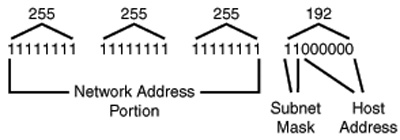
Figure 24.4. A subnet mask can be used to identify the network address, subnet address, and host portions of the IP address.

The first thing you should do when preparing to subnet an address space is decide how many host addresses will be needed on each subnet. Then convert this number to its binary value. Looking at the binary value, you can see how many bits you will need for the host portion of the address space. If you then subtract that value from the number of bits available (which is 8 if you’re subnetting the last byte of a Class C address), you can calculate what the decimal equivalent would be for a binary number that contains that number of leftmost bits set to one.

Suppose you wanted to create subnets that would allow you to put up to 30 computers on each subnet. First, determine what 30 is when converted to binary: 11110. You can see that it takes 5 bits to represent the decimal value of 30 in binary. After you subtract this from 8, you have left only 3 bits that can be “borrowed” from the Class C host part of the address (8 – 5 = 3). In binary, this mask would be 11100000. If you convert this value to decimal, you get 224.

The next question to ask is how many subnets can you create using this mask? Because only 3 bits are left, just figure out the largest number you can express using 3 bits in binary. You’ll come up with a value of all 1s (111), which translates to 7 in decimal. Therefore, you can have seven possible subnets, or eight if you include zero as a possibility.

After you’ve calculated what your subnet mask needs to be, you’ll need to calculate what the actual host addresses must be for each subnet. The first subnet address would be 000. Because the IP address is expressed in dotted decimal notation, calculate how many addresses you can store in an 8-bit binary value that always begins with 000, and then translate that to decimal: 00000001 to 00011110, which is 1–30 in decimal.

Continuing the process, the second subnet address would be 001, and the third would be 011. The range of host addresses that could be created for a subnet value of 001 is 00100001 to 00111110, which is 33–62 in decimal.

The range of hosts on the second subnet would be from 192.113.255.33 to 192.113.255.62.

Simply continue this process and you’ll be able to figure out the correct subnet addresses, based on the mask you’ve chosen.

It’s possible to further divide the Class C address space by using up to 6 bits for the subnet mask, but this would leave only two usable host addresses and is not very practical. However, it can be done!

Classless Interdomain Routing Notation and Supernetting

As we discussed earlier in this chapter, the system of classifying IP addresses (A, B, C) worked well when the Internet was much smaller. The class system and subnetting is still widely used on local network routers. However, on the Internet backbone routers, a system called Classless Interdomain Routing (CIDR) is the method used to determine where to route a packet. This technique is also referred to as supernetting. CIDR can be considered a technique that uses a subnet mask that ignores the traditional IP class categories.

Why is CIDR needed? When the IP address class system was introduced, it was simple for routers to use the first byte of the IP address to figure out the network number, and thus make routing an easy task. For example, for an IP address of 140.176.232.333, the router would recognize that 140 falls in the Class B address range, so the network number would be 140.176.0. A quick glance at the routing table was all that was necessary to determine the next hop to which a packet should be routed to get to its network.

As the Internet continued to grow (or explode, as some might say), the huge number of Class B and Class C networks that were being added meant that routing tables on Internet backbone routers were also growing at a fast rate. Eventually, there would come a point where it would be impossible to efficiently route packets if routing tables continued to grow.

CIDR allows for address aggregation. That is, a single entry in a routing table can represent many lower-level network addresses.

Another reason why CIDR was needed is that much of the classful address space is wasted. This happens at both ends of the spectrum. Consider a small network at the low end, with a total of 254 usable addresses in a Class C address block. If the owner of that address space has a network with only 50 or 100 computers, that means that more than half of the available host addresses are essentially lost to the Internet. At the high end, a Class A network has a total of 16,777,216 possible host addresses. How many organizations need 16 million host addresses?

By dropping the address class constraints, and instead using a subnet mask to specify any number of contiguous bits of the IP address as the network address, it is possible to carve up the total 32-bit address space into finer blocks that can be allocated more efficiently.

CIDR uses a specific notation to indicate which part of the IP address is the network portion and which is the host portion. The CIDR notation syntax is the network address followed by /#, where # is a number indicating how many bits of the address represent the network address. This /# is commonly called the network prefix. Table 24.6 shows the network prefix values for A, B, and C network classes.

Table 24.6. CIDR Network Prefix Notation for A, B, and C IP Address Classes

However, because CIDR no longer recognizes classes, it’s quite possible to have a network address like 140.176.123.0/24. Thus, while 140 would indicate that only 16 bits are used as the network portion of the address when using classful addressing, the /24 notation would specify that the first 24 bits are used, and the remaining 8 bits would be used for host addressing. Using the /24 notation allows the former class B address space to be allocated in smaller blocks than the class system allows.

In Table 24.7 you can see how this system allows for networks that range in size from 32 hosts to more than 500,000 hosts. The middle column shows the equivalent of a Class C network address space that the CIDR prefix creates, and the last column shows the number of hosts that would exist in the network.

Table 24.7. Use of CIDR Network Prefix Notations

In Table 24.7, note that I’ve expressed the Class C equivalent networks that can be created. However, when using the /16 prefix, you get 256 Class C size networks, which is the same thing as a single Class B network. To continue this train of thought, a /15 prefix will allow you to create two Class B–sized networks, and so on.

Using CIDR, blocks of addresses can be allocated to ISPs that in turn subdivide the address space efficiently when they create address spaces for clients. One drawback is that a network that is composed completely of CIDR routing would require, in order to operate most efficiently, that addresses remain with the ISP under which a particular block is owned. This means that if your company decides to move to a different ISP, you would most likely have to obtain a new address block and therefore have to reconfigure your network addresses. If you use Network Address Translation and a private address space on your internal corporate network, this would be only a minimal problem.

Another problem with CIDR is that some host clients might not support it. That is, if the TCP/IP stack recognizes the different classes, it might not operate if you try to configure it using a subnet mask that does not match the traditional Class A, B, or C values. Again, because most routers do support this capability, you can solve this problem by using the CIDR addresses for your routers and using NAT and a private address space for the internal network.

The Address Resolution Protocol—Resolving IP Addresses to Hardware Addresses

As just discussed, IP provides a logical hierarchical address space that makes routing data from one network to another a simple task. When the datagram arrives at the local subnet, however, another protocol comes into play. The Address Resolution Protocol (ARP) is used to resolve the IP address to the hardware, to the address of the workstation, or to another network device that is the target destination of the datagram. Whereas IP addresses are used to allow for routing between networks or network segments, ARP is used at the end of the road for the final delivery.

It is important to understand that when devices communicate directly on the local network segment (on the wire, so to speak), the actual address used to communicate between two devices, whether they are computers, routers, or whatever, is the built-in Media Access Control (MAC) address. In the case of two hosts on the same subnet, ARP can quickly resolve the correct address translations, and communications take place quickly and efficiently. When a router stands between two computers, the actual hardware address that the computer communicates with is the MAC address of the router, not of the computer that lies at the end of the connection. Using Ethernet as an example, when a datagram needs to be routed to another network or subnet, the computer sends the datagram to the default route, sometimes called the default gateway, which is the router that connects the network segment to the rest of the world (or the rest of the corporate network).

The router then consults its routing tables and decides on the next device that the packet needs to get to on its way to its destination. Sometimes this is simply a computer that is connected on another segment that is also connected to the router. Sometimes it is several more routers that the packet must pass through. However, when the packet finally reaches the network segment on which the target computer is located, ARP is used by the router to find out the MAC address of the computer that is configured with the IP address found inside the packet.

To get this MAC address, a computer or router will first send out a broadcast message that every computer on the local segment can see. This ARP message contains the sending computer’s own MAC address and also the IP address of the computer to which it wants to talk. When a computer recognizes its IP address in this broadcast packet, it sends a packet that contains its own MAC address back to the computer that originated the ARP message. After that, both computers know the MAC address of the other, and further transmissions take place using these hardware addresses.

The actual fields in the ARP broadcast frame are listed here:

Hardware Type—This is a 2-byte field that identifies the kind of hardware used at the data-link layer of the sending computer. For diagnostic purposes, Table 24.8 contains a list of the most common hardware types.

Protocol Type—This is a 2-byte field that specifies the protocol type of the address that the computer wants to translate to a hardware address.

Hardware Address Length—This is a 1-byte field that specifies the length of the source and destination hardware address fields that will follow.

Protocol Address Length—Similarly, this 1-byte field specifies the length of the source and destination protocol address fields that will follow in this packet.

Opcode—This 1-byte field is used to determine the type of ARP frame. Frame types are listed in Table 24.9.

Sender Hardware Address—This variable-length field (as defined by the Hardware Address Length field) contains the sending computer’s hardware (MAC) address.

Sender Protocol Address—This variable-length field (as defined by the Protocol Address Length field) contains the sender’s protocol address—an IP address, for example.

Target Hardware Address—This variable-length field (as defined by the Hardware Address Length field) contains the destination computer’s hardware (MAC) address.

Target Protocol Address—This variable-length field (as defined by the Protocol Address Length field) contains the protocol address that the sender wants to resolve to a hardware address.

Table 24.8. Hardware Type Field Values

As you can see from this table, the Address Resolution Protocol is not limited to just resolving IP addresses on a standard Ethernet network. It has been extended over time to accommodate many kinds of networking technologies. Some of the entries in Table 24.8 are dinosaurs—extinct protocols that no longer are being marketed. This list will probably continue to grow, however, as newer technologies are developed.

Table 24.9 shows that the Opcode field also has a large number of values, some of which might at first appear quite strange. For example, the MARS entries are not used for resolving addresses for strange spacecraft that appear in the sky now and then. They are used for address resolution on ATM networks where multicasting is being used.

Table 24.9. Opcodes for ARP Frames

For more information about ATM, see Chapter 15, “Dedicated Connections.” For more information about MARS, see RFC 2022, “Support for Multicast Over UNI 3.0/3.1 Based ATM Networks.”

The InARP entries in Table 24.9 are used for Inverse ARP. This form of ARP is used when the underlying network technology is a nonbroadcast multiple access (NBMA) type, such as an X.25, ATM, or Frame Relay network. In these types of networks, a virtual circuit identifier is used instead of a hardware address. RFC 2390 contains the details about InARP and how it is used in a Frame Relay network to find out the IP address when only the virtual circuit identifier is known. Finally, you will also see entries in the table that correspond to Reverse ARP, which is discussed in the next section.

To prevent a storm of broadcast messages that would result if this were done for each packet that needed to be delivered on the local network segment, each host keeps a table, or cache, of MAC addresses in memory for a short time. When it becomes necessary to communicate with another computer, this ARP cache is first checked. If the destination address is not found in the ARP cache, the ARP broadcast method is used.

Figure 24.5 demonstrates how IP addresses are used during the routing process, while hardware addresses are used for the actual device-to-device communications.

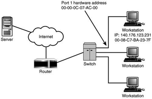
Figure 24.5. The IP address routes the datagram through the network, while the hardware addresses are used between individual workstations and devices on the network.

If the server in this figure wants to send a packet to the workstation with the IP address 140.176.123.231, it will quickly realize that this address is not on the local subnet and will send the IP packet, perhaps encapsulated in an Ethernet frame, to its default gateway. The gateway, which is connected to the Internet, uses the IP address to route the packet to the local router for the workstation. When the router receives the packet, it consults its routing tables and finds the switch (or hub) that is connected to the network segment by comparing the network portion of the IP address to entries in the routing table. When the packet finally arrives at the switch, the switch consults a table of MAC hardware addresses to look up the hardware address of the destination computer. From then on, communications between the workstation and the switch use these hardware addresses for actual communication.

In fact, every device, from the server shown later in Figure 24.6 to the router to the switch, and all the devices that lie in between on the Internet, uses the MAC address for communications. The IP address information is used by routers to deliver the packet to the next hop the packet must take to get to the final destination local segment. The MAC addresses are used for device-to-device communication. The ARP protocol is used to find out the hardware address at each hop, unless it’s already stored in the ARP cache.

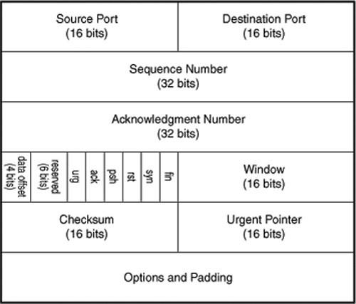
Figure 24.6. The TCP protocol header fields also can be used for filtering packets.

The arp command (which is found in most Unix and Windows operating systems) lets you view the ARP table. It also can be used to add or delete entries in the table. Although the syntax varies between different systems, the following should work for most:

arp -a—Displays the current contents of the arp table.

arp -d IP_address—Deletes the entry for the specified host.

arp -s IP_address ethernet_address—Adds an entry to the table.

For example, to add an entry use the following syntax:

arp -s 192.113.121.88   08-00-2b-34-c1-01

Using the few commands in this list will help you become more familiar with how ARP works. Examine the contents of your local table. Then, try pinging several other systems and examine the table again to see whether entries for those systems have been added to the table. Wait a few minutes and check the table again to see whether the entries have timed out.

Proxy ARP

Sometimes, different network segments both use the same network ID and are connected by a router or another device. Because ARP uses broadcast packets to resolve IP addresses to hardware addresses, it would appear that computers on different network segments that use the same network ID would never be able to communicate.

Proxy ARP allows for just such a situation. The router or other device that connects the physical network segments is configured to provide the proxy ARP service. When a host broadcasts an ARP packet to learn the hardware address of a device that is on a different physical segment, the ARP proxy device recognizes this situation and acts as a go-between. The proxy device responds to the ARP broadcast and sends the originating computer a datagram that contains the proxy device’s IP address instead of the actual target computer’s IP address. From that point on, the host that originated the ARP request will communicate with the host on the other segment by sending packets to the proxy device, which will know to forward them to the computer on the other subnet.

Another use of proxy ARP comes into play for remote access servers. For example, when users dial into a computer that is acting as a remote access server, they are communicating with software on the remote access server and are not actually physically connected to the subnet. The remote access server recognizes this and will intercept any ARP broadcast packets that are trying to resolve the dial-in computer’s IP address. Communications then take place between the host on the local subnet and the remote computer through the remote access server. The host on the local subnet sends unicast packets to the remote access server, which forwards them to the remote client.

Yet another use for proxy ARP is to support older systems that use a TCP/IP stack that doesn’t understand subnetting or those that use the older method for broadcast packets—a host address of all zeros instead of the current standard of all ones. Although this is not really much of a problem today, you might still find older legacy systems that cannot be abandoned, yet they cannot properly interact with newer systems when you subnet your network. The solution for this is to place the older systems on a separate network segment and let the proxy ARP device take care of resolving protocol addresses.

RARP—The Reverse Address Resolution Protocol

The Reverse Address Resolution Protocol (RARP) does just what it sounds like it would do. It performs the opposite function of ARP. It is most commonly used by diskless workstations that need to discover what their IP address is when they boot. Because the diskless workstation already knows its hardware address (because the address is burned into the network card), the workstation uses RARP to send a broadcast packet requesting that a server respond to its request by sending it an ARP frame containing an IP address it can use.

Note that the same packet format is used for ARP and RARP. The Opcode field is used to indicate what kind of operation is being performed.

The Transmission Control Protocol (TCP)

As we have discussed so far, the IP protocol is a protocol that can be used to make a best-effort attempt to get a packet from one host to another, even when the hosts are on different networks. The Transmission Control Protocol uses IP but adds functionality that makes TCP a reliable, connection-oriented protocol. Whereas IP doesn’t require any acknowledgment that a packet is ever received, TCP does. Whereas IP does no preliminary communication with the target system to set up any kind of session, TCP does. TCP builds on the functions that IP provides to create a session that can be used by applications for a reliable exchange of data. As stated earlier in this chapter, IP is similar to sending a letter in the mail. TCP can be compared to the “return receipt requested” function which acknowledges that the letter was received by someone at the destination address. One interesting difference, however, is that TCP doesn’t necessarily need an acknowledgment for each packet sent. Instead, it is possible for a single acknowledgment to be sent in response to more than one IP packet.

TCP Provides a Reliable Connection-Oriented Session

Whereas IP provides a checksum mechanism in its header to ensure that the IP header is not corrupted during transit, the TCP protocol provides checksums on the data that is transmitted. TCP also has mechanisms that regulate the flow of data to avoid problems associated with congestion. TCP also uses sequence numbers in the TCP header so that IP packets can be reassembled in the correct order on the receiving end of the communication.

Examining TCP Header Information

Each layer in the TCP/IP protocol stack adds information to the data it receives from a layer above it. This process is usually called encapsulation, and the added data is usually called a header. The header information is significant only to the layer that adds it, and it is added as a message is passed down the stack and stripped off at the destination as the packet is passed back up the protocol stack. Some layers also add data at the end of the packet. This is called a trailer.

Earlier we looked at the makeup of the IP header. In Figure 24.6 you can see the layout of the TCP header. This header information is sometimes referred to as the TCP Protocol Data Unit.

Remember that TCP is responsible for establishing a reliable connection-oriented session between two applications across a network. TCP receives data (called messages) from layers above it in the protocol stack, adds its own header information, and then passes it to the IP layer, which then adds its own header information. The messages sent to TCP from applications up the stack are usually called a stream of data, because the amount of data can vary and is not limited to a set number of bytes. TCP takes these messages and, if they are too large to fit into a packet, breaks them into smaller segments and sends each segment in a separate packet. The TCP layer at the receiving end reassembles these messages before passing them up to an application.

Whereas most of the header information we looked at in the IP header was used for routing the packet through the Internet, the information in the TCP header is concerned with other issues, such as reliability of the connection and ordering of the messages being sent. The header fields for TCP include these:

Source port—This 16-bit field is used to identify the port being used by the application that is sending the data. Ports are discussed in more detail later in this chapter.

Destination port—This 16-bit field is used to identify the port to which the packet will be delivered on the receiving end of the connection.

Sequence number—This 32-bit field is used to identify where a segment fits in the larger message when a message is broken into fragments for transmission.

Acknowledgment number—This 32-bit field is used to indicate what the next sequence number should be. That is, this value is the next byte in the data stream that the receiver expects to receive from the sender.

Data offset—This 4-bit field is used to specify the number of 32-bit words that make up the header. This field is used to calculate the start of the data portion of the packet.

Reserved—These 6 bits were reserved for future use and, because they were never generally used, are supposed to be set to zeros.

URG flag—When this bit is set to 1, the field titled Urgent Pointer will point to a section of the data portion of the packet that is flagged as “urgent.”

ACK flag—This is the acknowledgment bit. If it’s set to 1, the packet is an acknowledgment. If it’s set to 0, the packet is not an acknowledgment.

PSH flag—If this bit is set to 1, it indicates a push function; otherwise, it is set to 0.

RST flag—If this bit is set to 1, it is a signal that the connection is to be reset; otherwise, it is set to 0.

SYN flag—If this bit is set to 1, it indicates that the sequence numbers are to be synchronized. If it’s set to 0, the sequence numbers are not to be synchronized.

FIN flag—If this bit is set to 1, it specifies that the sender is finished sending information; otherwise, it is set to 0.

Window—This 16-bit field is used to specify how many blocks of data the receiving computer is able to accept at this time.

Checksum—This 16-bit field is a calculated value used to verify the integrity of both the header and the data portions of the packet.

Urgent pointer—If the URG flag is set, this 16-bit field points to the offset from the sequence number field into the data portion of the packet where the urgent data is stored. TCP does not use this field itself, but applications above TCP in the stack might do so.

Options—This field can be of variable length and is similar to the Options field in the IP header. One function this field is used for is to specify the maximum segment size.

Because the Options field can vary, the header is padded with extra bits so that it will be a multiple of 32 bits.

The amount of information stored in the TCP header makes it possible to use the protocol for complex communications. TCP can implement error checking, flow control, and other necessary mechanisms to ensure reliable delivery of data throughout the network. However, because of the complexity of this header, hackers can use many different methods to manipulate the TCP protocol when trying to gain access to your network or otherwise cause you problems.

One interesting thing to note about the checksum field is that it is calculated based on three things:

The TCP header fields

The TCP data

Pseudo header information

The pseudo header information consists of the source and destination IP addresses, one byte set to all zeros, an 8-bit protocol field, and a 16-bit field that contains the length of the TCP segment. The address and protocol fields are duplicated from the IP packet, and the length field is redundant because it also is contained in the TCP header. Because the algorithm used to calculate the checksum is based on 16-bit words, the TCP packet may be padded with a zero byte for calculation purposes only. If the checksum field contains a value of zero, this indicates that no checksum was calculated by the sender. If by some chance the value of the checksum results in a value of zero, the checksum field is set to all 1s (65,535 decimal).

TCP Sessions

Because TCP is a connection-oriented protocol, the computers that want to communicate must first establish the conditions that will govern the session and set up the connection. TCP allows for twoway communication—that is, it’s a bidirectional, full-duplex connection. Both sides can send and receive data at the same time. To set up a connection, each side must “open” its side of the connection. On the server side this is called a passive open. The server application runs as a process on the server computer and listens for connection requests coming in for a certain port. For example, the Telnet server process typically listens for connections on port 23. By using both the IP address and a port number, the server process can uniquely identify each client that makes a connection request. Ports are discussed in more detail later in this chapter.

When a client computer wants to establish a connection to a server, it goes through a process known as an active open. The server is already listening for connection requests (passive open), but the client must initiate the actual connection process by sending a request to the port number of the server application it wants to use.

In Figure 24.7 (shown in the next section), the single-bit field named SYN is the “synchronization” bit. You also can see in Figure 24.7 another field titled ACK, for the acknowledgment bit. These 2 bits are very important and are used during the process of setting up a TCP/IP session so that a reliable connection can be established between two computers on the network.

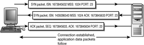
Figure 24.7. TCP uses a three-way handshake to establish a connection.

Setting Up a TCP Session

A TCP/IP connection is made between two computers, using their addresses and, depending on the application using TCP, port numbers. The SYN and ACK bits in the TCP header are important components used to establish this initial connection.

The steps involved in setting up a TCP/IP connection appear in Figure 24.7 and are listed here:

1. The client sends a TCP segment to the server with which it wants to establish a connection. The TCP header SYN field (“synchronize”) is set indicating that it wants to synchronize sequence numbers so that further exchanges can be identified as belonging to this particular connection and so that the segments sent can be reassembled into the correct order and acknowledged. This first initial sequence number in the TCP header is set to an initial value chosen by the TCP software on the client computer. Additionally, the port-number field in the TCP header is set to a value of the port on the server to which the client wants to connect. Port numbers can be thought of as representing the application to which the computer wants to connect.

2. When the server receives this segment, it returns a segment to the client with the SYN field set. The server’s segment also contains an initial sequence number, which is chosen by its TCP software implementation. To show the client that it received the initial connection segment, the ACK bit is also set, and the acknowledgment field contains the client’s initial sequence number, incremented by 1.

3. The client, upon receiving this acknowledgment from the server, sends another segment to the server, acknowledging the server’s initial sequence number. This is done in the same manner in which the server acknowledges the client’s initial sequence number. The acknowledgment field contains the server’s initial sequence number incremented by a value of 1.

During this exchange, the 16-bit acknowledgment field is incremented by 1. You might wonder why the acknowledging computer doesn’t just send back the same sequence number it received from the sending computer. It increments the sequence number that it received to indicate the next sequence number it expects to receive from the sending computer. Thus, during each exchange of TCP segments, each side is telling the other side what it is expecting to get from the other side during the next transmission. The sequence numbers are used to indicate the next byte in the data stream that the receiving end of the connection expects to receive. Thus, when the actual data exchange begins to take place, the sequence numbers are not simply incremented by a value of 1, but instead they are set to the actual number of bytes received (offset from the initial sequence number chosen for the connection) plus 1.

Because three segments are used in this process, the connection setup is often referred to as a three-way handshake. In the last of these three steps the SYN bit is not set, because the segment is simply acknowledging the server’s initial sequence number. Note also that port numbers are used to indicate the application for which the connection is being set up. TCP headers don’t need to contain the source and destination IP addresses because that information is already stored in the IP datagram that encapsulates the TCP message.

The method used to choose values for the initial sequence number can vary from one implementation of TCP to another. However, there are two important points to understand about the sequence numbers:

1. For each connection a client makes to another computer, the initial sequence number for each connection must be unique. If the same initial sequence number were used for every connection the client made to a single server, it would be impossible to differentiate between different connections of the same application (that is, port number) between the two machines. Although the IP address and port number can uniquely identify a computer, they can’t uniquely identify multiple applications of the same process running on the same computer.
2. Sequence numbers are incremented for each segment exchanged and are acknowledged by the receiver so that both sides can determine that segments are being delivered reliably and not getting lost in the network. However, it is not necessary that each and every segment be acknowledged with another segment. Using a technique called sliding windows (which we’ll get to in a moment), TCP allows for a single acknowledgment of a number of segments.

In Figure 24.7 another field is also shown in the first two packets that are exchanged. The Maximum Segment Size (MSS) field in the TCP header indicates the maximum number of bytes of data that the sender wants to receive in each TCP segment. This value is used to help prevent fragmentation of the TCP segment as it travels through various network devices that might have different transmission frame sizes. This value applies only to the size of the data that the TCP segment carries, and does not include the bytes that make up the TCP and IP headers. You will see this field only during the connection setup. After the application data exchange begins, this field is not used. If the client or server does not put a value into this field during the connection setup, a default value, usually 536, is used.

Not shown in this figure is the TCP field that stores the window size. This field is used to help manage the connection after the application data exchange begins.

Managing the Session Connection

After a TCP session has been established between two computers, the application that uses TCP can begin to communicate with its counterpart on the other computer. TCP receives a stream of bytes (called a message) from an application and stores them in a buffer. When the buffer is full, or when the application indicates that it wants TCP to send the message to the destination computer, the bytes are assembled into a TCP segment with the necessary TCP header information, and the segment is passed to IP for transmission on the network.

Each transmission was acknowledged during the initial connection setup. This is not always the case when the actual exchange of data begins between two computers. Instead, there are several important mechanisms that TCP uses to manage a connection after it has been established. These include

TCP timers

Sliding windows

Retransmissions

When a segment is passed to the IP layer for transmission, a timer is set and a countdown starts. When this retransmission timer reaches zero with no acknowledgment, the sending computer assumes that the segment did not make it to its destination and retransmits the segment. This function requires that TCP keep data in a memory buffer until it is acknowledged.

During the connection setup, each side of the connection indicates to the other side the maximum amount of data it can buffer in memory. This is the window size. This value indicates how many TCP segments the computer can receive before an acknowledgment is required. For example, on a Windows 2000 client the default value for this field when using Ethernet for transmission is 12 segments.

Another feature of TCP that helps to reduce the number of packets transmitted is the fact that the acknowledgment of received data does not have to travel in a packet separate from those that hold data. In other words, when sending data in a TCP segment to the remote computer, the sending computer also can use the ACK bit and the sequence number fields to acknowledge data that it has received from the remote computer. This is sometimes called a piggyback ACK because both data and an acknowledgment of data received travels in the same packet.

Having sliding windows also helps to reduce the number of packets transmitted by allowing a single acknowledgment to be sent for multiple segments. Instead of acknowledging every single segment that it receives, the receiver can send an acknowledgment that indicates the last byte received when it receives several contiguous segments in a short time. That is, the acknowledgment can be cumulative. Each end of the connection uses a send and receive buffer to store data received or waiting for transmission.

Remember that the application which uses TCP passes a stream of bytes to TCP or receives a stream of bytes from TCP, depending on the direction in which data is flowing at any particular point in time. The term sliding window refers to the fact that the receiving buffer can hold only so much data (the window size advertised by the receiving end). The amount of space available in the buffer can change over time, depending on the amount of time it takes for the application to accept the bytes from TCP and thus make more room in the buffer. The receiving end can use the window size TCP header field to tell the sender the number of bytes it can currently receive and store in its buffer. This window size is called the offered window size. That doesn’t mean that the sender must send that amount of data, just that the receiver is ready to accept any number of data bytes, up to that size.

As you can see in Figure 24.8, the sender can calculate the amount of data it can send by comparing the window size offered, the bytes already sent and acknowledged, and the bytes that have been sent but not acknowledged. In this figure the window size offered by the receiver is 4 bytes. Because 2 bytes have already been sent and the window size is four, the sender can transmit 2 more bytes at this time. As bytes are acknowledged by the receiver, the left edge of the window slides toward the right, as shown in this figure. Depending on how well the receiving end of the connection is able to process incoming bytes, the offered window size can change, which in turn can affect the number of bytes that the sending end can transmit. As the buffer empties at the receiving end, a larger window size can be advertised and the right edge of the window slides toward the right.

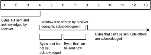
Figure 24.8. The window size advertised by the receiver of TCP segments determines which bytes in the data stream the sender can transmit.

It also is possible that the buffer at the receiving end becomes full, and the sender is sent a window size that is now zero. The sender will not send any more segments until the window size is offered again at a value greater than zero.

Using this scheme, there are several things to keep in mind. First, the sender does not have to send an amount of data that is equal to the size of the offered window. It can send less. Second, the receiver does not have to wait until it has received data in the amount of the offered window before it sends an acknowledgment. Third, the window size is controlled, under most circumstances, by the receiving end of the connection.

In this example we have used a transmission that consists of only a few bytes at a time. For most TCP communications the amount of data, and the window size, is much larger.

Sliding windows tell the sender when and how much data it can transmit. When a connection is initially established, a technique called slow start is used to govern the amount of data that is sent, allowing it to increase to a point that the particular network will tolerate. When a connection has been in use for some time, congestion can occur and it might be necessary to slow down the rate at which segments are transmitted, by using a technique called the congestion avoidance algorithm. These two methods work together to control the flow of data during the connection.

Slow start means that when the transmitting side of a connection first transmits data, it does so by observing how fast it receives acknowledgments of data from the receiving end. A variable in the TCP software keeps track of the congestion window (cwnd), which is initially set to one segment. For each segment that is acknowledged, the cwnd variable is incremented. Then, the sender is allowed to send an amount of data up to the value of cwnd or the size of the offered window, whichever is the lower value. As you can see, the faster the receiving end acknowledges segments, the larger the cwnd variable becomes, and thus the more segments that the sender will be able to transmit (up to the offered window size). The offered window size enables the receiving end to control the amount of data that can be sent. The congestion window gives the sending end of the transmission control over how much data can be transmitted. Thus, both sides work together to throttle up data transmissions, starting off slowly, until the receiver is unable to buffer data at a faster rate or until network congestion forces the connection to operate at a slower rate.

The term slow start isn’t actually an accurate way to describe what happens. In reality, the receiving end might acknowledge several segments, thus increasing the size of cwnd by more than one when it sends a single acknowledgment to account for multiple segments. This means that, instead of being incremented by one for each acknowledgment, cwnd can be incremented at a much faster rate. However, this method does allow for TCP to “test the waters,” so to speak, to determine the rate at which data can be sent, up to the receiving end’s capacity to buffer data and pass it up to the application on its end of the connection.

As packets make their way through the network, however, another problem can arise. In today’s world, communications often take place between computers that reside on different networks that are connected by routers, and we find that, just like the freeway system, congestion can occur when too many computers are trying to send and receive data at the same time. When a router or another network connection device becomes a bottleneck, it can simply drop IP packets—remember that IP is an unreliable protocol. It is up to TCP to realize what is happening and to compensate for it by retransmitting unacknowledged segments.

The retransmission timer that we discussed earlier is used by the transmitting end of the connection to determine when a segment should be retransmitted. This value is recalculated over time, depending on the round-trip time it takes for a transmission to make it to the receiving end and an acknowledgment to get back to the transmitting side of the connection. The round-trip time can change over time, depending on the amount of data flowing through the network. Round-trip time also can change when the routes chosen by routers change, thus sending packets through a different path in the network that can take more or less time than previous transmissions.

The congestion avoidance algorithm is used to take care of situations in which the network becomes congested and packets are dropped—that is, they are not being acknowledged by the receiver. Although this algorithm is separate from the slow start technique, in practice they work together. In addition to the cwnd variable, another variable called the slow start threshold size (ssthresh) comes into play. This variable is initially set to 65,535 bytes when a connection is established. When congestion is detected, the value of this variable is set to half the currently offered window size, and the variable cwnd is set to the value of one maximum segment size (MSS)—though this can vary from one implementation to another. In recent Microsoft operating systems including Windows 2000 and Windows XP, cwnd is set to the value of two times the MSS. The send window value then is set to the lower of the cwnd and the offered receive window size.

Based on which value is chosen, TCP segments are then sent. If the segments are acknowledged, cwnd is incremented. If the value of cwnd is lower than the value of ssthresh, a slow start is used. When the value of cwnd is equal to half the current offered window size from the receiving end of the transmission, congestion avoidance is used. Remember that the value of ssthresh can be used to determine this because it recorded the value of the offered window size (divided by two) that was in effect when congestion started.

During congestion avoidance, the value of cwnd is incremented by one cwnd for each acknowledgment received—again, this value might be different according to your particular TCP implementation. Thus, instead of a possible exponential increase that a slow start method would allow, congestion avoidance allows for a smaller increase in the value of cwnd. After all, if congestion is occurring, the last thing you want to do is quickly increase the rate of transmission. Instead, you want to throttle it up more slowly. So although slow start will increment cwnd by the number of segments acknowledged by a single acknowledgment, the congestion avoidance algorithm will increment cwnd by only one segment for each acknowledgment received, no matter how many segments are being acknowledged by the acknowledgment.

Other mechanisms are used for flow control in TCP, such as the fast recovery algorithm and the fast retransmit algorithm. Discussing these topics is beyond the scope of this book. The important thing to understand is that TCP does monitor and adjust its transmissions, from both sides of the connection, to try to get the maximum amount of data flowing without causing problems. It’s a self-regulating protocol, you might say.

Ending a TCP Session

When the party’s over—the application is finished sending data to another computer—it tells TCP to close the connection from its side. Because the connection must be closed from each end, this is called a half-close. To fully close a TCP connection, four steps are required, as opposed to the threeway handshake method used to set up the connection. Four steps are required because TCP operates as a full-duplex connection—that is, data can flow in both directions. Thus, each side needs to tell the other side of the connection that it has finished sending data and wants to close the connection.

For example, when the client application, such as Telnet, wants to close a connection, TCP sends a segment that has the FIN bit set in the TCP header to the remote computer. The remote computer must first acknowledge this FIN segment, and does so by sending a segment to the client that has the ACK bit set. Because the connection is full-duplex, the server TCP software informs the Telnet server application that the user application on the other end of the connection is finished. It then sends its own FIN segment to the client, which, as you can probably guess, sends an acknowledgment segment back to the server.

Although this is the general method used to close a TCP connection, another technique can be used in which one side sends a FIN segment, closing its data pipe, but the other side of the connection does not. Instead, it is possible for the other side to continue sending data until it is finished, at which time it sends the FIN segment and waits for an acknowledgment, which effectively closes the connection.

A good example of this method is the Unix rsh (remote shell) utility. This utility allows a user to execute a command on a remote server. Because Unix allows for the capability to redirect input (using the < operator), a user can use rsh to execute a command on a remote server, and use the < operator on the command line to redirect the input for the command from the command line to a file. In such a situation, the client’s side of the connection sends the command to be executed to the remote server and then starts sending the data that is in the file. After the client’s side of the connection finishes sending the data contained in the file to the remote server, it instructs TCP to close its side of the connection. Yet, at the other side of the connection, the data needs to be processed by the program invoked by the rsh command. When finished, the program on the remote server sends the data back to the client and then instructs TCP to close its side of the connection.

TCP Session Security Issues

Calling TCP a reliable protocol means that it uses an acknowledgment mechanism to ensure that the data is received at the remote computer intact. Reliable does not mean that TCP is a secure protocol. If that were so, there would be no need for firewalls! Although the connection setup and termination methods used to create a connection create a virtual circuit between the two computers, there are many ways to exploit TCP (and IP) to break into a computer. For example, every time a new connection is requested on a server (the receipt of a TCP segment with the SYN bit set), the computer sets aside data structures in memory to store information about the connection it is setting up. This requires a few CPU cycles and memory on the computer.

It should be obvious that an easy way to cause a “denial of service” attack against a computer is to simply send a large number of SYN segments to it in a short period. If the number of SYN segments and the rate at which they are sent exceed the capacity of the CPU or memory of the server, then, depending on the operating system and how the TCP/IP stack is implemented, the system might slow to a crawl or crash.

For more information about how the inner workings of TCP/IP and related protocols can be used maliciously, see Chapter 44, “Security Issues for Wide Area Networks.” For information on how to protect yourself against these sorts of attacks, see Chapter 45.

The User Datagram Protocol (UDP)

Although TCP uses an acknowledgment mechanism to ensure that data is actually delivered to another computer, the User Datagram Protocol (UDP) does not. Both use IP as a transport protocol, but UDP is a much simpler protocol that doesn’t require the overhead that TCP does. If an application does not need the benefits that a TCP connection provides, UDP can be used. Because UDP does no session setup, and all UDP datagrams are independent entities on the network, it can be considered an unreliable, connectionless protocol.

An example of this is the Domain Name Service (DNS). Most implementations of DNS use UDP packets in order to efficiently exchange information with other computers. If a client doesn’t receive a response back from a simple DNS request, it can try again, or simply use another DNS server if it is configured to do so.

Examining UDP Header Information

Compared to the TCP header, the UPD header is much smaller because it doesn’t require fields for sequence or acknowledgment numbers. UDP also doesn’t need the connection setup flags, window size fields, and other information required for a connection-oriented protocol. In Figure 24.9 you can see that UDP has only four fields.

Figure 24.9. The UPD protocol uses a smaller header.

The following are the purposes of the UDP header fields:

Source port—This 16-bit field is used to identify the port being used by the application that is sending the data.

Destination port—This 16-bit field is used to identify the port to which the packet will be delivered on the receiving end of the connection.

Length—This 16-bit field is used to store the length of the entire UDP datagram, which includes both the header and data portions.

Checksum—This 16-bit field is used to ensure that the contents of the UDP datagram are not corrupted in transit.

Although the length field in the UDP header can store a value of up to 65,535, in actual practice the size of a datagram is usually limited to a much smaller value. For example, the application programming interface (API) of a particular operating system might use smaller fields to specify the length of a datagram.

The checksum field is calculated on the UDP header information and its data, along with pseudo header information, just as is done with TCP. Using this method, UDP can determine whether the IP layer has passed to it a datagram that was not intended for this computer. If the checksum calculated on the receiving end does not match the value stored in this field, the UDP datagram is discarded. Similar to IP, no message is sent back to the sender of the datagram if this happens. For a reliable connection an application should use TCP, not UDP.

Interaction Between UDP and ICMP

Whereas UDP has no built-in mechanisms for guaranteeing delivery of the information carried in its datagrams, the Internet Control Message Protocol (ICMP) is used to report conditions back to the sending computer. For example, if a UDP datagram is sent to a computer with a destination port that is not being used (that is, that service is not running on the destination computer), then the ICMP port unreachable message (subcode value 3 of the destination unreachable message) is returned to the sender.

ICMP messages also can be used with UDP to find out the maximum transmission unit (MTU) size—that is, the largest size a datagram can be in order to be sent through the network without being fragmented. Remember that on a network that uses different routers, or perhaps on an internetwork that is made up of different types of equipment or network media, the maximum size of a frame can change from one device to another. To discover the maximum size of a datagram that can be sent through the network, another subcode of the ICMP unreachable message (subcode 4) can be used along with UDP.

To create a utility that can be used to discover the MTU of a network connection, the IP Don’t Fragment field can be set in the IP header information. When the UDP datagram reaches a router or other device that can’t forward the datagram without fragmenting it, it will return the ICMP unreachable message “fragmentation needed, don’t fragment bit set.”

Finally, in some implementations a router or host will return the ICMP “source quench” error if a system is sending UDP datagrams at a rate that is too fast for the system receiving them. In this case, the application using UDP should be coded to take this into account, because the datagrams will be discarded by the system that generates the “source quench” ICMP messages.

Ports, Services, and Applications

If all applications that used the network only identified the destination for their data exchange as a single IP address, the information would arrive at the destination computer, but it would be almost impossible for the targeted system to figure out which process to give the data to.

Both the TCP and the UDP protocols use port numbers to solve this problem. Each application that communicates on the network using TCP/IP also specifies a port number on the target computer. The port numbers are endpoints for the communications path so that two applications communicating across the network can identify each other. Think of a street address for a business. If all the mail arrived simply addressed with the street address, how would you determine who should get each letter? A person’s name or the suite or room number is used so that the endpoint of the communication becomes more fully defined. This is how ports work.

For example, suppose you’ve established a Telnet session with a remote computer and decide you want to download a file to that computer. Telnet doesn’t transfer files, so you would have to open an FTP connection. Because the source and destination addresses would be the same in the IP packet for both of these sessions, port numbers are used to indicate the application.

When you combine an address with a port number, you have an identifier that can uniquely identify both endpoints of a communication. The name used for this combination of numbers is a socket. This is illustrated in Figure 24.10, in which two computers have established two communication sessions, one for Telnet (port 23) and one for FTP (port 20). FTP actually uses two ports—port 20 for sending data and port 21 for exchanging command information.

Figure 24.10. A socket is composed of an address and port number, and uniquely identifies an endpoint of a network connection.

It should quickly become apparent to you why a packet filter would find these port numbers useful. Instead of having to permit or deny packets based only on their source or destination address—and thereby allow or disallow all communications—it is possible to selectively allow or disallow individual services. Although you might not want your users to Telnet to a remote host computer (or vice versa), you might not care if they exchange files through anonymous FTP sessions. By using port numbers in packet filtering rules, you can enable or disable network services one at a time.

Well-Known Ports

The Internet Corporation for Assigned Names and Numbers (ICANN) is the organization that controls the first range of port numbers that are available (0–1023), and these are usually called “well-known ports.” The use for these ports has been defined in several RFCs, most recently RFC 1700. However, in January 2002, RFC 3232, “Assigned Numbers: RFC 1700 Is Replaced by an On-line Database,” made RFC 1700 obsolete. Instead, RFC 3232 is a simple memo which states that port numbers will be maintained in an online database that you can access via the IANA Web site.

Well-known ports are usually accessible on a given system by a privileged process or privileged users. For example, the FTP utility uses ports 20 and 21, whereas the Telnet utility uses port 23. In most cases the User Datagram Protocol (UDP) and Transmission Control Protocol (TCP) make the same use of a particular port. This is not required, however. Understanding the application that a port is used for can be useful when deciding which ports to block when building a firewall. Some of these applications will never be used by your system, and because of that, there exists no good reason to allow network traffic through the firewall that uses these ports.

Registered Ports

Ports numbered from 1024 to 65535 also can be used but are not reserved by IANA. These ports are called registered ports and can be used by most any user process on the system.

The Internet Control Message Protocol (ICMP)

The Internet Control Message Protocol is a required part of any TCP/IP implementation, and the functions it performs are very important to routers and other network devices that communicate through TCP/IP. Like TCP and UPD, this protocol also uses the IP protocol to send its messages through the network. If you have used the ping or traceroute commands, you have used ICMP. ICMP was first defined in RFC 792.

Whereas TCP can usually recover from dropped datagrams simply by requesting that IP retransmit them, ICMP is used as a reporting mechanism that can be used by IP (and thus the protocols that use IP).

There are many kinds of ICMP messages, but all share a similar format. These are the fields of an ICMP message:

Type—This 1-byte field is used to indicate the kind of ICMP message (see Table 24.10).

Code—This 1-byte field is used as a subcode to further identify a message. This field is set to zero if the particular message type does not need to be further delineated.

Checksum—This 2-byte field is used to provide an error-checking code for the entire ICMP message.

Type-Specific Data—This field can vary in length and is used to provide further data specific to the ICMP message type.

Table 24.10. ICMP Message Types

ICMP Message Types

Table 24.10 shows the different types of messages that make up ICMP. The numbers listed in the Message Type field are what will be found in the Type field of the ICMP message.

The ping command uses the echo request and echo reply messages to determine whether a physical connection exists between systems. Another important function on the Internet is traffic control, and the source quench message can be sent to tell a sending host that the destination host cannot keep up with the speed at which it is sending packets. The transmitting computer can keep sending these quench messages until the sender scales back its transmissions to an acceptable rate.

A router uses another valuable function ICMP (the Redirect Message) to tell another router that it knows of a better path to a destination. Routers also can use the time-exceeded messages to report to another device as to why a packet was discarded.

Routers are not the only devices that use ICMP. Host computers can use ICMP. For example, when a computer boots and does not know what the network mask is for the local LAN, it can generate an address mask request message. Another device on the network can reply to assist the computer.

The Code field in the ICMP message is used for only some of the ICMP message types. The Destination Unreachable message has the largest number of code types. Table 24.11 lists these codes.

Table 24.11. ICMP Message Codes

As you can see, ICMP can be used to compose quite detailed messages to indicate error conditions, offer advice on routing possibilities, and perform other functions that help make the Internet easier to manage.

Some situations will cause an ICMP message to not be generated. For example, ICMP messages are never created in response to an error in another ICMP message. That doesn’t mean that ICMP messages can’t be created in response to other ICMP messages, however. For example, the echo request and echo reply messages work together in a query/response format. Other instances that usually don’t generate ICMP messages include these:

IP broadcast and multicast messages

Link-layer broadcast messages (that is, Ethernet frame broadcast messages)

Datagrams that have a source address that is not for a unique host, such as the loopback address

Messages that have been fragmented, except for the first fragment

If ICMP messages were allowed to correct problems with multicast or broadcast messages, a large number could be generated, causing the problem to become worse. This is the reason for most of the preceding conditions limiting the use of ICMP.

For the most part, the use of ICMP is described in other sections of this book where their use is employed. For example, Chapter 27 discusses using ICMP to implement the traceroute and ping commands. Some of these messages are not discussed in this book, either because they are no longer used (as indicated in the table) or because their use is trivial or rare.