
Packet Classification
Traditionally, the post office forwards messages based on the destination address in each letter. Thus all letters to Timbuctoo were forwarded in exactly the same way at each post office. However, to gain additional revenue, the post office introduced service differentiation between ordinary mail, priority mail, and express mail. Thus forwarding at the post office is now a function of the destination address and the traffic class. Further, with the spectre of terrorist threats and criminal activity, forwarding could even be based on the source address, with special screening for suspicious sources.
In exactly the same way, routers have evolved from traditional destination-based forwarding devices to what are called packet classification routers. In modern routers, the route and resources allocated to a packet are determined by the destination address as well as other header fields of the packet, such as the source address and TCP/UDP port numbers.
Packet classification unifies the forwarding functions required by firewalls, resource reservations, QoS routing, unicast routing, and multicast routing. In classification, the forwarding database of a router consists of a potentially large number of rules on key header fields. A given packet header can match multiple rules. So each rule is given a cost, and the packet is forwarded using the least-cost matching rule.
This chapter is organized as follows. The packet classification problem is motivated in Section 12.1. The classification problem is formulated precisely in Section 12.2, and the metrics used to evaluate rule schemes are described in Section 12.3. Section 12.4 presents simple schemes such as linear search and CAMs. Section 12.5 begins the discussion of more efficient schemes by describing an efficient scheme called grid of tries that works only for rules specifying values of only two fields. Section 12.6 transitions to general rule sets by describing a set of insights into the classification problem, including the use of a geometric viewpoint.
Section 12.7 begins the transition to algorithms for the general case with a simple idea to extend 2D schemes. A general approach based on divide-and-conquer is described in Section 12.8. This is followed by three very different examples of algorithms based on divide-and-conquer: simple and aggregated bit vector linear search (Section 12.9), cross-producting (Section 12.10), and RFC, or equivalenced cross-producting (Section 12.11). Section 12.12 presents the most promising of the current algorithmic approaches, an approach based on decision trees.
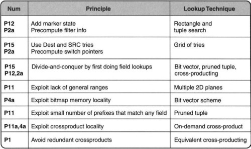
This chapter will continue to exhibit the set of principles introduced in Chapter 3, as summarized in Figure 12.1. The chapter will also illustrate three general problem-solving strategies: solving simpler problems first before solving a complex problem, collecting different viewpoints, and exploiting the structure of input data sets.
12.1 WHY PACKET CLASSIFICATION?
Packet forwarding based on a longest-matching-prefix lookup of destination IP addresses is fairly well understood, with both algorithmic and CAM-based solutions in the market. Using basic variants of tries and some pipelining (see Chapter 11), it is fairly easy to perform one packet lookup every memory access time.
Unfortunately, the Internet is becoming more complex because of its use for mission-critical functions executed by organizations. Organizations desire that their critical activities not be subverted either by high traffic sent by other organizations (they require QoS guarantees) or by malicious intruders (they require security guarantees). Both QoS and security guarantees require a finer discrimination of packets, based on fields other than the destination. This is called packet classification. To quote John McQuillan [McQ97]:
Routing has traditionally been based solely on destination host numbers. In the future it will also be based on source host or even source users, as well as destination URLs (universal resource locators) and specific business policies…. Thus, in the future, you may be sent on one path when you casually browse the Web for CNN headlines. And you may be routed an entirely different way when you go to your corporate Web site to enter monthly sales figures, even though the two sites might be hosted by the same facility at the same location…. An order entry form may get very low latency, while other sections get normal service. And then there are Web sites comprised of different servers in different locations. Future routers and switches will have to use class of service and QoS to determine the paths to particular Web pages for particular end users. All this requires the use of layers 4, 5, and above.
This new vision of forwarding is called packet classification. It is also sometimes called layer 4 switching, because routing decisions can be based on headers available at layer 4 or higher in the OSI architecture. Examples of other fields a router may need to examine include source addresses (to forbid or provide different service to some source networks), port fields (to discriminate between traffic types, such as Napster and E-mail), and even TCP flags (to distinguish between externally and internally initiated connections). Besides security and QoS, other functions that require classification include network address translation (NAT), metering, traffic shaping, policing, and monitoring.
Several variants of packet classification have already established themselves on the Internet. First, many routers implement firewalls [CB95] at trust boundaries, such as the entry and exit points of a corporate network. A firewall database consists of a series of packet rules that implement security policies. A typical policy may be to allow remote login from within the corporation but to disallow it from outside the corporation.
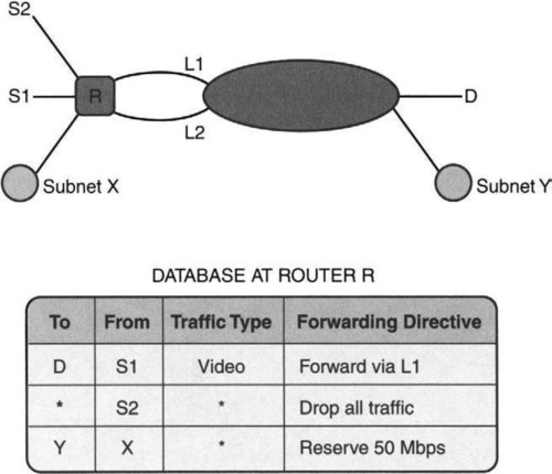
Second, the need for predictable and guaranteed service has led to proposals for reservation protocols, such as DiffServ [SWG], that reserve bandwidth between a source and a destination. Third, the cries for routing based on traffic type have become more strident recently — for instance, the need to route Web traffic between Site 1 and Site 2 on, say, Route A and other traffic on, say, Route B. Figure 12.2 illustrates some of these examples.
Classifiers historically evolved from firewalls, which were placed at the edges of networks to filter out unwanted packets. Such databases are generally small, containing 10–500 rules, and can be handled by ad hoc methods. However, with the DiffServ movement, there is potential for classifiers that could support 100,000 rules for DiffServ and policing applications at edge routers.
While large classifiers are anticipated for edge routers to enforce QoS via DiffServ, it is perhaps surprising that even within the core, fairly large (e.g., 2000-rule) classifiers are commonly used for security. While these core router classifiers are nowhere near the anticipated size of edge router classifiers, there seems no reason why they should not continue to grow beyond the sizes reported in this book. For example, many of the rules appear to be denying traffic from a specified subnetwork outside the ISP to a server (or subnetwork) within the ISP. Thus, new offending sources could be discovered and new servers could be added that need protection. In fact, we speculate that one reason why core router classifiers are not even bigger is that most core router implementations slow down (and do not guarantee true wire speed forwarding) as classifier sizes increase.
12.2 PACKET-CLASSIFICATION PROBLEM
Traditionally, the rules for classifying a message are called rules and the packet-classification problem is to determine the lowest-cost matching rule for each incoming message at a router.
Assume that the information relevant to a lookup is contained in K distinct header fields in each message. These header fields are denoted H[1], H[2], …, H[K], where each field is a string of bits. For instance, the relevant fields for an IPv4 packet could be the destination address (32 bits), the source address (32 bits), the protocol field (8 bits), the destination port (16 bits), the source port (16 bits), and TCP flags (8 bits). The number of relevant TCP flags is limited, and so the protocol and TCP flags are combined into one field — for example, TCP-ACK can be used to mean a TCP packet with the ACK bit set.1 Other relevant TCP flags can be represented similarly; UDP packets are represented by H[3] = UDP.
Thus, the combination (D, S, TCP-ACK, 63, 125) denotes the header of an IP packet with destination D, source S, protocol TCP, destination port 63, source port 125, and the ACK bit set.
The classifier, or rule database, router consists of a finite set of rules, R1, R2, …, RN. Each rule is a combination of K values, one for each header field. Each field in a rule is allowed three kinds of matches: exact match, prefix match, and range match. In an exact match, the header field of the packet should exactly match the rule field — for instance, this is useful for protocol and flag fields. In a prefix match, the rule field should be a prefix of the header field — this could be useful for blocking access from a certain subnetwork. In a range match, the header values should lie in the range specified by the rule — this can be useful for specifying port number ranges.
Each rule Ri, has an associated directive dispi which specifies how to forward the packet matching this rule. The directive specifies if the packet should be blocked. If the packet is to be forwarded, the directive specifies the outgoing link to which the packet is sent and, perhaps, also a queue within that link if the message belongs to a flow with bandwidth guarantees.
A packet P is said to match a rule R if each field of P matches the corresponding field of R — the match type is implicit in the specification of the field. For instance, if the destination field is specified as 1010*, then it requires a prefix match; if the protocol field is UDP, then it requires an exact match; if the port field is a range, such as 1024–1100, then it requires a range match. For instance, let R = (1010*, *, TCP, 1024–1080, *) be a rule, with disp = block. Then, a packet with header (10101 …111, 11110… 000, TCP, 1050, 3) matches R and is therefore blocked. The packet (10110… 000, 11110… 000, TCP, 80, 3), on the other hand, doesn’t match R.
Since a packet may match multiple rules in the database, each rule R in the database is associated with a nonnegative number, cost(R). Ambiguity is avoided by returning the least-cost rule matching the packet’s header. The cost function generalizes the implicit precedence rules that are used in practice to choose between multiple matching rules. In firewall applications or Cisco ACLs, for instance, rules are placed in the database in a specific linear order, where each rule takes precedence over a subsequent rule. Thus, the goal there is to find the first matching rule. Of course, the same effect can be achieved by making cost(R) equal to the position of rule R in the database.
As an example of a rule database, consider the topology and firewall database [CB95] shown in Figure 12.3, where a screened subnet configuration interposes between a company subnetwork (shown on top left) and the rest of the Internet (including hackers). There is a so-called bastion host M within the company that mediates all access to and from the external world. M serves as the mail gateway and also provides external name server access. TI, TO are network time protocol (NTP) sources, where TI is internal to the company and TO is external. S is the address of the secondary name server, which is external to the company.
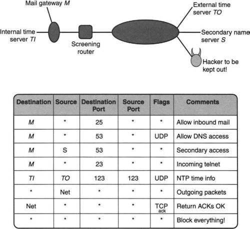
Clearly, the site manager wishes to allow communication from within the network to TO and S and yet wishes to block hackers. The database of rules shown on the bottom of Figure 12.3 implements this intention. Terse explanations of each rule are shown on the right of each rule. Assume that all addresses of machines within the company’s network start with the CIDR prefix Net. Thus M and TI both match the prefix Net. All packets matching any of the first seven rules are allowed; the remaining (last rule) are dropped by the screening router. A more general firewall could arbitrarily interleave rules that allow packets with rules that drop packets.
As an example, consider a packet sent to M from S with UDP destination port equal to 53. This packet matches Rules 2, 3, and 8 but must be allowed through because the first matching rule is Rule 2.
Note that this description uses N for the number of rules and K for the number of packet fields. K is sometimes called the number of dimensions, for reasons that will become clearer in Section 12.6.
12.3 REQUIREMENTS AND METRICS
The requirements for rule matching are similar to those for IP lookups (Chapter 11). We wish to do packet classification at wire speed for minimum-size packets, and thus speed is the dominant metric. To allow the database to fit in high-speed memory it is useful to reduce the amount of memory needed. For most firewall databases, insertion speed is not an issue because rules are rarely changed.
However, this is not true for dynamic or stateful packet rules. This capability is useful, for example, for handling UDP traffic. Because UDP headers do not contain an ACK bit that can be used to determine whether a packet is the bellwether packet of a connection, the screening router cannot tell the difference between the first packet sent from the outside to an internal server (which it may want to block) and a response sent to a UDP request to an internal client (which it may want to pass). The solution used in some products is to have the outgoing request packet dynamically trigger the insertion of a rule (which has addresses and ports that match the request) that allows the inbound response to be passed. This requires very fast update times, a third metric.
12.4 SIMPLE SOLUTIONS
There are five simple solutions that are often used or considered: linear search, caching, demultiplexing algorithms, MPLS, and content addressable memories (CAMs). While CAMs have difficult hardware design issues, they effectively represent a parallelization of the simplest algorithmic approach: linear search.
12.4.1 Linear Search
Several existing firewall implementations do a linear search of the database and keep track of the best-match rule. Linear search is reasonable for small rule sizes but is extremely slow for large rule sets. For example, a core router that does linear search among a rule set of 2000 rules (used at the time of writing by some ISPs) will considerably degrade its forwarding performance below wire speed.
12.4.2 Caching
Some implementations even cache the result of the search keyed against the whole header. There are two problems with this scheme. First, the cache hit rate of caching full IP addresses in the backbones is typically at most 80–90% [Par96, NMH97]. Part of the problem is Web accesses and other flows that send only a small number of packets; if a Web session sends just five packets to the same address, then the cache hit rate is 80%. Since caching full headers takes a lot more memory, this should have an even worse hit rate (for the same amount of cache memory).
Second, even with a 90% hit rate cache, a slow linear search of the rule space will result in poor performance.2 For example, suppose that a search of the cache costs 100 nsec (one memory access) and that a linear search of 10,000 rules costs 1,000,000 nsec = 1 msec (one memory access per rule). Then the average search time with a cache hit rate of 90% is still 0.1 msec, which is rather slow. However, caching could be combined with some of the fast algorithms in this chapter to improve the expected search time even further. An investigation of the use of caching for classification can be found in Xu et al. [XSD00].
12.4.3 Demultiplexing Algorithms
Chapter 8 describes the use of packet rules for demultiplexing and algorithms such as Pathfinder, Berkeley packet filter, and dynamic path finder. Can’t these existing solutions simply be reused? It is important to realize that the two problems are similar but subtly different.
The first packet-classification scheme that avoids a linear search through the set of rules is Pathfinder [BGP+94]. However, Pathfinder allows wildcards to occur only at the end of a rule. For instance, (D, S, *, *, *) is allowed, but not (D, *, Prot, *, SourcePort). With this restriction, all rules can be merged into a generalized trie — with hash tables replacing array nodes — and rule lookup can be done in time proportional to the number of packet fields. DPF [EK96] uses the Pathfinder idea of merging rules into a trie but adds the idea of using dynamic code generation for extra performance. However, it is unclear how to handle intermixed wildcards and specified fields, such as (D, *, Prot, *, SourcePort), using these schemes.
Because packet classification allows more general rules, the Pathfinder idea of using a trie does not work well. There does exist a simple trie scheme (set-pruning tries; see Section 12.5.1) to perform a lookup in time O(M), where M is the number of packet fields. Such schemes are described in Decasper et al. [DDPP98] and Malan and Jahanian [MJ98]. Unfortunately, such schemes require Θ(NK) storage, where K is the number of packet fields and N is the number of rules. Thus such schemes are not scalable for large databases. By contrast, some of the schemes we will describe require only O(NM) storage.
12.4.4 Passing Labels
Recall from Chapter 11 that one way to finesse lookups is to pass a label from a previous-hop router to a next-hop router. One of the most prominent examples of such a technology is multiprotocol label switching (MPLS) [Cha97]. While IP lookups have been able to keep pace with wire speeds, the difficulties of algorithmic approaches to packet classification have ensured an important niche for MPLS. Refer to Chapter 11 for a description of tag switching and MPLS.
Today MPLS is useful mostly for traffic engineering. For example, if Web traffic between two sites A and B is to be routed along a special path, a label-switched path is set up between the two sites. Before traffic leaves site A, a router does packet classification and maps the Web traffic into an MPLS header. Core routers examine only the label in the header until the traffic reaches B, at which point the MPLS header is removed.
The gain from the MPLS header is that the intermediate routers do not have to repeat the packet-classification effort expended at the edge router; simple table lookup suffices. The DiffServ [SWG] proposal for QoS is actually similar in this sense. Classification is done at the edges to mark packets that deserve special quality of service. The only difference is that the classification information is used to mark the Type of Service [TOS] bits in the IP header, as opposed to an MPLS label. Both are examples of Principle P10, passing hints in protocol headers.
Despite MPLS and DiffServ, core routers still do classification at the very highest speeds. This is largely motivated by security concerns, for which it may be infeasible to rely on label switching. For example, Singh et al. [SBV04] describe a number of core router classifiers, the largest of which contains 2000 rules.
12.4.5 Content-Addressable Memories
Recall from Chapter 11 that a CAM is a content-addressable memory, where the first cell that matches a data item will be returned using a parallel lookup in hardware. A ternary CAM allows each bit of data to be either a 0, a 1, or a wildcard. Clearly, ternary CAMs can be used for rule matching as well as for prefix matching. However, the CAMs must provide wide lengths — for example, the combination of the IPv4 destination, source, and two port fields is 96 bits.
Because of problems with algorithmic solutions described in the remainder of this chapter, there is a general belief that hardware solutions such as ternary CAMs are needed for core routers, despite the problems [GM01] of ternary CAMs. There are, however, several reasons to consider algorithmic alternatives to ternary CAMs, which were presented in Chapter 11.
Recall that these reasons include the smaller density and larger power of CAMs versus SRAMs and the difficulty of integrating forwarding logic with the CAM. These problems remain valid when considering CAMs for classification. An additional issue that arises is the rule multiplication caused by ranges. In CAM solutions, each range has to be replaced by a potentially large number of prefixes, thus causing extra entries. Some algorithmic solutions can handle ranges in rules without converting ranges to rules.
These arguments are strengthened by the fact that, at the time of writing, several CAM vendors were also considering algorithmic solutions, motivated by some of the difficulties with CAMs. While better CAM cell designs that reduce density and power requirements may emerge, it is still important to understand the corresponding advantages and disadvantages of algorithmic solutions. The remainder of the chapter is devoted to this topic.
12.5 TWO-DIMENSIONAL SCHEMES
A useful problem-solving technique is first to solve a simpler version of a complex problem such as packet classification and to use the insight gained to solve the more complex problem. Since packet classification with just one field has been solved in Chapter 11, the next simplest problem is two-dimensional packet classification.
Two-dimensional rules may be useful in their own right. This is because large backbone routers may have a large number of destination–source rules to handle virtual private networks and multicast forwarding and to keep track of traffic between subnets. Further, as we will see, there is a heuristic observation that reduces the general case to the two-dimensional case.
Since there are only three distinct approaches to one-dimensional prefix matching — using tries, binary search on prefix lengths, and binary search on ranges — it is worth looking for generalizations of each of these distinct approaches. All three generalizations exist. However, this chapter will describe only the most efficient of these (the generalization of tries) in this section.
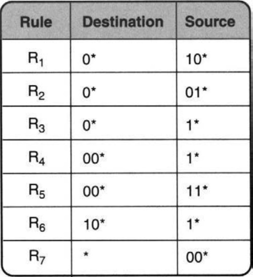
The appropriate generalization of standard prefix tries to two dimensions is called the grid of tries. The main idea will be explained using an example database of seven destination–source rules, shown in Figure 12.4. We arrive at the final solution by first considering two naive variants.
12.5.1 Fast Searching Using Set-Pruning Tries
Consider the two-dimensional rule set in Figure 12.4. The simplest idea is first to build a trie on the destination prefixes in the database and then to hang a number of source tries off the leaves of the destination trie. Figure 12.5 illustrates the construction for the rules in Figure 12.4. Each valid prefix in the destination trie points to a trie containing some source prefixes. The question is: Which source prefixes should be stored in the source trie corresponding to each destination prefix?
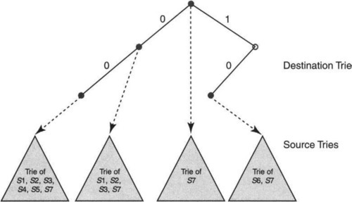
For instance, consider D = 00*. Both rules R4 and R5 have this destination prefix, and so the trie at D clearly needs to store the corresponding source prefixes 1* and 11*. But storing only these source prefixes is insufficient. This is because the destination prefix 0* in rules R1, R2, and R3 also matches any destination that D matches. In fact, the wildcard destination prefix * of R7 also matches whatever D matches. This suggests that the source trie at D = 00 must contain the source prefixes for {R1, R2, R3, R4, R5, R7}, because these are the set of rules whose destination is a prefix of D.
Figure 12.5 shows a schematic representation of this data structure for the database of Figure 12.4. Note that S1 denotes the source prefix of rule R1, S2 of rule R2, and so on. Thus each prefix D in the destination trie prunes the set of rules from the entire set of rules down to the set of rules compatible with D. The same idea can be extended to more than two fields, with each field value in the path pruning the set of rules further.
In this trie of tries, the search algorithm first matches the destination of the header in the destination trie. This yields the longest match on the destination prefix. The search algorithm then traverses the associated source trie to find the longest source match. While searching the source trie, the algorithms keep track of the lowest-cost matching rule. Since all rules that have a matching destination prefix are stored in the source trie being searched, the algorithm finds the correct least-cost rule. This is the basic idea behind set-pruning trees [Decasper et al., DDPP98].
Unfortunately, this simple extension of tries from one to two dimensions has a memory-explosion problem. The problem arises because a source prefix can occur in multiple tries. In Figure 12.5, for instance, the source prefixes S1, S2, S3 appear in the source trie associated with D = 00* as well as the trie associated with D = 0*.
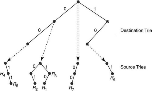
How bad can this replication get? A worst-case example forcing roughly N2 memory is created using the set of rules shown in Figure 12.6. The problem is that since the destination prefix * matches any destination header, each of the N/2 source prefixes are replicated N/2 times, one for each destination prefix. The example (see exercises) can be extended to show a O(Nk) bound for general set-pruning tries in K dimensions.
While set-pruning tries do not scale to large classifiers, the natural extension to more than two fields has been used in Decasper et al. [DDPP98] as part of a router toolkit, and in Malan and Jahanian [MJ98] as part of a flexible monitoring system. The performance of set-pruning tries is also studied in Qiu et al. [QVS01]. One interesting optimization introduced in Decasper et al. [DDPP98] and Malan and Jahanian [MJ98] is to avoid obvious waste (P1) when two subtries S1 and S2 have exactly the same contents. In this case, one can replace the pointers to S1 and S2 by a pointer to a common subtrie, S. This changes the structure from a tree to a directed acyclic graph (DAG). The DAG optimization can greatly reduce storage for set-pruning tries (see Ref. QVS01 for other, related optimizations) and can be used to implement small classifiers, say, up to 100 rules, in software.
12.5.2 Reducing Memory Using Backtracking
The previous scheme pays in memory in order to reduce search time. The dual idea is to pay with time in order to reduce memory. In order to avoid the memory blowup of the simple trie scheme, observe that rules associated with a destination prefix D are copied into the source trie of D′ whenever D is a prefix of D′. For instance, in Figure 12.5, the prefix D = 00* has two rules associated with it: R4 and R5. The other rules, R1, R2, R3, are copied into D’s trie because their destination field 0* is a prefix of D.
The copying can be avoided by having each destination prefix D point to a source trie that stores the rules whose destination field is exactly D. This requires modifying the search strategy as follows: Instead of just searching the source trie for the best-matching destination prefix D, the search algorithm must now search the source tries associated with all ancestors of D.
In order to search for the least-cost rule, the algorithm first traverses the destination trie and finds the longest destination prefix D′ matching the header. The algorithm then searches the source trie of D′ and updates the least-cost-matching rule. Unlike set-pruning tries, however, the search algorithm is not finished at this point.
Instead, the search algorithm must now work its way back up the destination trie and search the source trie associated with every prefix of D′ that points to a nonempty source trie.3
Since each rule now is stored exactly once, the memory requirement for the new structure is O(NW), which is a significant improvement over the the previous scheme. Unfortunately, the lookup cost for backtracking is worse than for set-pruning tries: In the worst case, the lookup costs Θ(W2), where W is the maximum number of bits specified in the destination or source fields.
The Θ(W2) bound on the search cost follows from the observation that, in the worst case, the algorithm may end up searching W source tries, each at the cost of O(W), for a total of O(W2) time. For W = 32 and using 1-bit tries, this is 1024 memory accesses. Even using 4-bit tries, this scheme requires 64 memory accesses.
While backtracking can be very slow in the worst case, it turns out that all classification algorithms exhibit pathological worst-case behavior. For databases encountered in practice, backtracking can work very well. Qiu et al. [QVS01] describe experimental results using backtracking and also describe potential hardware implementations on pipelined processors.
12.5.3 The Best of Both Worlds: Grid of Tries
The two naive variants of two-dimensional tries pay either a large price in memory (set-pruning tries) or a large price in time (backtracking search). However, a careful examination of backtracking search reveals obvious waste (P1), which can be avoided using precomputation (P2a).
To see the wasted time in backtracking search, consider matching the packet with destination address 001 and source address 001 in Figure 12.7. The search in the destination trie gives D = 00 as the best match. So the backtracking algorithm starts its search for the matching source prefix in the associated source trie, which contains rules R4 and R5. However, the search immediately fails, since the first bit of the source is 0. Next, backtracking search backs up along the destination trie and restarts the search in the source trie of D = 0*, the parent of 00*.
But backing up the trie is a waste because if the search fails after searching destination bits 00 and source bit 0, then any matching rule must be shorter in the destination (e.g., 0) and must contain all the source bits searched so far, including the failed bit. Thus backing up to the source trie of D = 0* and then traversing the source bit 0 to the parent of R2 in Figure 12.7 (as done in backtracking search) is a waste.
The algorithm could predict that this sequence of bits would be traversed when it first failed in the source trie of D = 00. This motivates a simple idea: Why not jump directly to the parent of R2 from the failure point in the source trie of D = 00*?
Thus in the new scheme (Figure 12.8), for each failure point in a source trie, the trie-building algorithm precomputes what we call a switch pointer. Switch pointers allow search to jump directly to the next possible source trie that can contain a matching rule. Thus in Figure 12.8, notice that the source trie containing R4 and R5 has a dashed line labeled with 0 that points to a node x in the source trie containing {R1, R2, R3}. All the dashed lines in Figure 12.8 are switch pointers. Please distinguish the dashed switch pointers from the dotted lines that connect the destination and source tries.
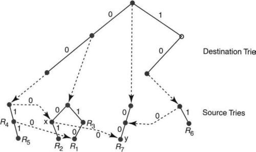
Now consider again the same search for the packet with destination address 001 and source address 001 in Figure 12.8. As before, the search in the destination trie gives D = 00 as the best match. Search fails in the corresponding source trie (containing R4 and R5) because the source trie contains a path only if the first source bit is a 1. However, in Figure 12.8, instead of failing and backtracking, the algorithm follows the switch pointer labeled 0 directly to node x. It then continues matching from node x, without skipping a beat, using the remaining bits of the source.
Since the next bit of the source is a 0, the search in Figure 12.8 fails again. The search algorithm once again follows the switch pointer labeled 0 and jumps to node y of the third source trie (associated with the destination prefix *). Effectively, the switch pointers allow skipping over all rules in the next ancestor source trie whose source fields are shorter than the current source match. This in turn improves the search complexity from O(W2) to O(W).
It may help to define switch pointers more precisely. Call a destination string D′ an ancestor of D if D′ is a prefix of D. Call D′ the lowest ancestor of D if D′ is the longest prefix of D in the destination trie. Let T(D) denote the source trie pointed to by D. Recall that T(D) contains the source fields of exactly those rules whose destination field is D.
Let u be a node in T(D) that fails on bit 0; that is, if u corresponds to the source prefix s, then the trie T(D) has no string starting with, s0. Let D″ be the lowest ancestor of D whose source trie contains a source string starting with prefix, s0, say, at node v. Then we place a switch pointer at node u pointing to node v. If no such node v exists, the switch pointer is nil. The switch pointer for failure on bit 1 is defined similarly. For instance, in Figure 12.8, the node labeled x fails on bit 0 and has a switch pointer to the node labeled y.
As a second example, consider the packet header (00*, 10*). Search starts with the first source trie, pointed to by the destination trie node 00*. After matching the first source bit, 1, search encounters rule R4. But then search fails on the second bit. Search therefore follows the switch pointer, which leads to the node in the second trie labeled with R1. The switch pointers at the node containing R1 are both nil, and so search terminates. Note, however, that search has missed the rule R3 = (0*, 1*), which also matches the packet header. While in this case R3 has higher cost than R1, in general the overlooked rule could have lower cost.
Such problems can be avoided by having each node in a source trie maintain a variable storedRule. Specifically, a node v with destination prefix D and source prefix S stores in storedRule(v) the least-cost rule whose destination field is a prefix of D and whose source field is a prefix of S. With this precomputation, the node labeled with R1 in Figure 12.8 would store information about R3 instead of R1 if R3 had lower cost than R1.
Finally, here is an argument that the search cost in the final scheme is at most 2W. The time to find the best destination prefix is at most W. The remainder of the time is spent traversing the source tries. However, in each step, the length of the match on the source field increases by 1 — either by traversing further down in the same trie or by following a switch pointer to an ancestral trie. Since the maximum length of the source prefixes is W, the total time spent in searching the source tries is also W. The memory requirement is O(NW), since each of the N rules is stored only once, and each rule requires O(W) space.
Note that k-bit tries (Chapter 11) can be used in place of 1-bit tries by expanding each destination or source prefix to the next multiple of k. For instance, suppose k = 2. Then, in the example of Figure 12.8, the destination prefix 0* of rules R1, R2, R3 is expanded to 00 and 01. The source prefixes of R3, R4, R6, are expanded to 10 and 11. Using k-bit expansion, a single prefix can expand to 2k−1 prefixes. The total memory requirement grows from 2NW to NW2k/k, and so the memory increases by the factor 2k−1/k. On the other hand, the depth of the trie reduces to W/k, and so the total lookup time becomes O(W/k).
The bottom line is that by using multibit tries, the time to search for the best matching rule in an arbitrarily large two-dimensional database is effectively the time for two IP lookups.
Just as the grid of tries represents a generalization of familiar trie search for prefix matching, there is a corresponding generalization of binary search on prefix lengths (Chapter 11) that searches a database of two field rules in 2W hashes, where W is the length of the larger of the two fields. This is a big gap from the log W time required for prefix matching using binary search on prefix lengths. In the special case where the rules do not overlap, the search time reduces even further to log2 W, as shown in Warkhede et al. [WSV01a]. While these results are interesting theoretically, they seem to have less relevance to real routers, mostly because of the difficulties of implementing hashing in hardware.
12.6 APPROACHES TO GENERAL RULE SETS
So far this chapter has concentrated on the special case of rules on just two header fields. Before moving to algorithms for rules with more than two fields, this section brings together some insights that inform the algorithms in later sections. Section 12.6.1 describes a geometric view of classification that provides visual insight into the problem. Section 12.6.2 utilizes the geometric viewpoint to obtain bounds on the fundamental difficulty of packet classification in the general case. Section 12.6.3 describes several observations about real rule sets that can be exploited to provide efficient algorithms that will be described in subsequent sections.
12.6.1 Geometric View of Classification
A second problem-solving technique that is useful is to collect different viewpoints for the same problem. This section describes a geometric view of classification that was introduced by Lakshman and Staliadis [LS98] and independently by Adisehsu [Adi98].
Recall from Chapter 11 that we can view a 32-bit prefix like 00* as a range of addresses from 000… 00 to 001… 11 on the number line from 0 to 232. If prefixes correspond to line segments geometrically, two-dimensional rules correspond to rectangles (Figure 12.9), three-dimensional rules to cubes, and so on. A given packet header is a point. The problem of packet classification reduces to finding the lowest-cost box that contains the given point.
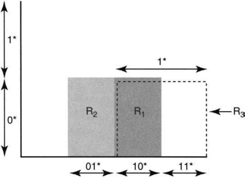
Figure 12.9 shows the geometric view of the first three two-dimensional rules in Figure 12.4. Destination addresses are represented on the y-axis and source addresses on the x-axis. In the figure, some sample prefix ranges are marked off on each axis. For example, the two halves of the y-axis are the prefix ranges 0* and 1*. Similarly, the x-axis is divided into the four prefix ranges 00*, 01*, 10*, and 11*. To draw the box for a rule like R1 = 0*, 10*, draw the 0* range on the y-axis and the 10* range on the x-axis, and extend the range lines to meet, forming a box. Multiple-rule matches, such as R1 and R2, correspond to overlapping boxes.
The first advantage of the geometric view is that it enables the application of algorithms from computational geometry. For example, Lakshman and Staliadis [LS98] adapt a technique from computational geometry known as fractional cascading to do binary search for two-field rule matching in O(log N) time, where N is the number of rules. In other words, twodimensional rule matching is asymptotically as fast as one-dimensional rule matching using binary search. This is consistent with the results for the grid of tries. The result also generalizes binary search on values for prefix searching as described in Chapter 11.
Unfortunately, the constants for fractional cascading are quite high. Perhaps this suggests that adapting existing geometric algorithms may actually not result in the most efficient algorithms. However, the second and main advantage of the geometric viewpoint is that it is suggestive and useful.
For example, the geometric view provides a useful metric, the number of disjoint (i.e., nonintersecting) classification regions. Since rules can overlap, this is not the number of rules. In two dimensions, for example, with N rules one can create N2 classification regions by having N/2 rules that correspond geometrically to horizontal strips together with N/2 rules that correspond geometrically to vertical strips. The intersection of the N/2 horizontal strips with the N/2 vertical strips creates O(N2) disjoint classification regions. For example, the database in Figure 12.6 has this property. Similar constructions can be used to generate O(NK) regions for K-dimensional rules.
As a second example, the database of Figure 12.9 has four classification regions: the rule R1, the rule R2, the points in R3 not contained in R1, and all points not contained in R1, R2, or R3. We will use the number of classification regions later to characterize the complexity of a given classifier or rule database.
12.6.2 Beyond Two Dimensions: The Bad News
The success of the grid of tries may make us optimistic about generalizing to larger dimensions. Unfortunately, this optimism is misplaced; either the search time or the storage blows up exponentially with the number of dimensions K for K > 2.
Using the geometric viewpoint just described, it is easy to adapt a lower bound from computational geometry. Thus, it is known that general multidimensional range searching over N ranges in k dimensions requires Ω((log N)K−1) worst-case time if the memory is limited to about linear size [Cha90b, Cha90a] or requires O(NK) size memory. While log N could be reasonable (say, 10 memory accesses), log4 N will be very large (say, 10,000 memory accesses). Notice that this lower bound is consistent with solutions for the two-dimensional cases that take linear storage but are as fast as O(log N).
The lower bound implies that for perfectly general rule sets, algorithmic approaches to classification require either a large amount of memory or a large amount of time. Unfortunately, classification at high speeds, especially for core routers, requires the use of limited and expensive SRAM. Thus the lower bound seems to imply that content address memories are required for reasonably sized classifiers (say, 10,000 rules) that must be searched at high speeds (e.g., OC-768 speeds).
12.6.3 Beyond Two Dimensions: The Good News
The previous subsection may have left the reader wondering whether there is any hope left for algorithmic approaches to packet classification in the general case. Fortunately, real databases have more structure, which can be exploited to efficiently solve multidimensional packet classification using algorithmic techniques.
The good news about packet classification can be articulated using four observations. Subsequent sections describe a series of heuristic algorithms, all of which do very badly in the worst case but quite well on databases that satisfy one or more of the assumptions.
The expected case can be characterized using four observations drawn from a set of firewall databases studied in Srinivasan et al. [SVSW98] and Gupta and McKeown [GM99b] (and not from publically available lookup tables as in the previous chapter). The first is identical to an observation made in Chapter 11 and repeated here. The observations are numbered starting from O2 to be consistent with observation O1 made in the lookup chapter.
O2: Prefix containment is rare. It is somewhat rare to have prefixes that are prefixes of other prefixes, as, for example, the prefixes 00* and 0001*. In fact, the maximum number of prefixes of a given prefix in lookup tables and classifiers is seven.
O3: Many fields are not general ranges. For the destination and source port fields, most rules contain either specific port numbers (e.g., port 80 for Web traffic), the wildcard range (i.e., *), or the port ranges that separate server ports from client ports (1024 or greater and less than 1024). The protocol field is limited to either the wildcard or (more commonly) TCP, UDP. This field also rarely contains protocols such as IGMP and ICMP. While other TCP fields are sometimes referred to, the most common reference is to the ACK bit.
O4: The number of disjoint classification regions is small. This is perhaps the most interesting observation. Harking back to the geometric view, the lower bounds in Chazelle [Cha90a] depend partly on the worst-case possibility of creating NK classification regions using N rules. Such rules require either NK space or a large search time. However, Gupta and McKeown [GM99b], after an extensive survey of 8000 rule databases, show that the number of classification regions is much smaller than the worst case. Instead of being exponential in the number of dimensions, the number of classification regions is linear in N, with a small constant.
O5: Source–Destination matching: In Singh et al. [BSV03], several core router classifiers used by real ISPs are analyzed and the following interesting observation is made. Almost all packets match at most five distinct source–destination values found in the classifier. No packet matched more than 20 distinct source–destination pairs. This is a somewhat more refined observation than O4 because it says that the number of classification regions is small, even when projected only to the source and destination fields. By “small,” we mean that the number of regions grows much more slowly than N, the size of the classifier.
12.7 EXTENDING TWO-DIMENSIONAL SCHEMES
The simplest general scheme uses observation O5 to trivially extend any efficient 2D scheme to multiple dimensions. A number of algorithms simply use linear search to search through all possible rules. This scales well in storage but poorly in time. The source–destination matching observation leads to a very simple idea depicted in Figure 12.10. Use source–destination address matching to reduce linear searching to just the rules corresponding to source–destination prefix pairs in the database that match the given packet header.
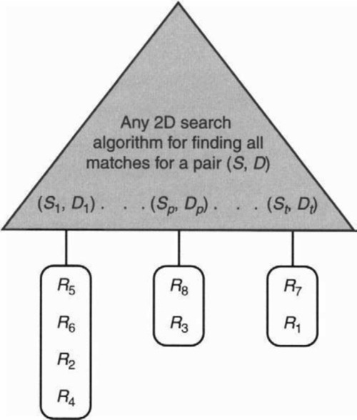
By observation O5, at most 20 rules match any packet when considering only the source and destination fields. Thus pruning based on source–destination fields will reduce the number of rules to be searched to less than 20, compared to searching the entire database. For example, Singh at al. [SBV04] describe a database with 2800 rules used by a large ISP.
Thus in Figure 12.10, the general idea is to use any efficient two-dimensional matching scheme to find all distinct source–destination prefix pairs (S1, D1)… (St, Dt) that match a header. For each distinct pair (Si, Di) there is a linear array or list with all rules that contain (Si, Di) in the source and destination fields. Thus in the figure, the algorithm has to traverse the list at (S1, D1), searching through all the rules for R5, R6, R2, and R4. Then the algorithm moves on to consider the lists at (S2, D2), and so on.
This structure has two important advantages:
• Each rule is represented only once without replication. However, one may wish to replicate rules to reduce search times even further.
• The port range specifications stay as ranges in the individual lists without the associated blowup associated with range translation in, say, CAMs.
Since the grid-of-tries implementation described earlier is one of the most efficient twodimensional schemes in the literature, it is natural to instantiate this general schema by using a grid of tries as the two-dimensional algorithm in Figure 12.10.
Unfortunately, it turns out that there is a delicacy about extending the grid of tries. In the the grid of tries, whenever one rule, R, is at least as specific in all fields as a second rule, R′, rule R′ precomputes its matching directive to be that of R if R is the lower cost of the two rules. This allows the traversal through the grid of tries to safely skip rule R when encountering rule R′. While this works correctly with two-field rules, it requires some further modifications to handle the general case.
One solution, equivalent to precomputing rule costs, is to precompute the list for R′ to include all the list elements for R. Unfortunately, this approach can increase storage because each rule is no longer represented exactly once. A more sophisticated solution, called the extended grid of tries (EGT) and described in Baboescu et al. [BSV03], is based on extra traversals beyond the standard grid of tries.
The performance of EGT can be described as follows.
Assumption: The extension of two-dimensional schemes depends critically on observation O5.
Performance: The scheme takes at least one grid-of-tries traversal plus the time to linearly search c rules, where c is the constant embodied in observation O5. Assuming linear storage, the search performance can increase [BSV03] by an additive factor representing the time to search for less specific rules. The addition of a new rule R requires only rebuilding of the individual two-dimensional structure of which R is a part. Thus rule update should be fairly fast.
12.8 USING DIVIDE-AND-CONQUER
The next three schemes (bit vector linear search, on-demand cross-producting, and equivalenced cross-producting) all exploit the simple algorithmic idea (P15) of divide-and-conquer. Divide-and-conquer refers to dividing a problem into simpler pieces and then efficiently combining the answers to the pieces. We briefly motivate a skeletal framework of this approach in this section. The next three sections will flesh out specific instantiations of this framework.
Chapter 11 has already outlined techniques to do lookups on individual fields. Given this background, the common idea in all three divide-and-conquer algorithms is the following. Start by slicing the rule database into columns, with the ith column storing all distinct prefixes (or ranges) in field i. Then, given a packet P, determine the best-matching prefix (or narrowest-enclosing range) for each of its fields separately. Finally, combine the results of the best-matching-prefix lookups on individual fields. The main problem, of course, lies in finding an efficient method for combining the lookup of individual fields into a single compound lookup.
All the divide-and-conquer algorithms conceptually start by slicing the database of Figure 12.3 into individual prefix fields. In the sliced columns, from now on we will sometimes refer to the wildcard character * by the string default. Recall that the mail gateway M and internal NTP agent TI are full IP addresses that lie within the prefix range of Net. The sliced database corresponding to Figure 12.3 is shown in Figure 12.11.
Clearly, any divide-and-conquer algorithm starts by doing an individual lookup in each column and then combines the results. The next three sections show that each of the three schemes returns different results with lookup and follows different strategies to combine the individual field results, despite using the same sliced database shown in Figure 12.11.
12.9 BIT VECTOR LINEAR SEARCH
Consider doing a match in one of the individual columns in Figure 12.11, say, the destination address field, and finding a bit string S as the longest match. Clearly, this lookup result eliminates any rules that do not match S in this field. Then the search algorithm can do a linear search in the set of all remaining rules that match S. The logical extension is to perform individual matches in each field; each field match will prune away a number of rules, leaving a remaining set. The search algorithm needs to search only the intersection of the remaining sets obtained by each field lookup.
This would clearly be a good heuristic for optimizing the average case if the remaining sets are typically small. However, one can guarantee performance even in the worst case (to some extent) by representing the remaining sets as bitmaps and by using wide memories to retrieve a large number of set members in a single memory access (P4a, exploit locality).
In more detail, as in Section 12.8, divide-and-conquer is used to slice the database, as in Figure 12.11. However, in addition with each possible value M of field i, the algorithm stores the set of rules S(M) that match M in field i as a bit vector. This is easy to do when building the sliced table. The algorithm that builds the data structure scans through the rules linearly to obtain the rules that match M using the match rule (e.g., exact, prefix, or range) specified for the field.
For example, Figure 12.12 shows the sliced database of Figure 12.11 together with bit vectors for each sliced field value. The bit vector has 8 bits, one corresponding to each of the eight possible rules in Figure 12.3. Bit j is set for value M in field i if value M matches Rule j in field i.
Consider the destination prefix field and the first value M in Figure 12.12. If we compare it to Figure 12.3, we see that the first four rules specify M in this field. The fifth rule specifies T1 (which does not match M), and the sixth and eighth rules specify a wildcard (which matches M). Finally, the seventh rule specifies the prefix Net (which matches M, because Net is assumed to be the prefix of the company network in which M is the mail gateway). Thus the bitmap for M is 11110111, where the only bit not set is the fifth bit. This is because the fifth rule has T1, which does not match M.
When a packet header arrives with fields H[1]… H[K], the search algorithm first performs a longest-matching-prefix lookup in each field i to obtain matches Mi, and the corresponding set S(Mi) of matching rules. The search algorithm then proceeds to compute the intersection of all the sets S(Mi) and returns the lowest-cost element in the intersection set.
But if rules are arranged in nondecreasing order of cost and all sets are bitmaps, then the intersection set is the AND of all K bitmaps. Finally, the lowest-cost element corresponds to the index of the first bit set in the intersection bitmap. But, the reader may object, since there are N rules, the intersected bitmaps are N bits long. Hence, computing the AND requires O(N) operations. So the algorithm is effectively doing a linear search after slicing and doing individual field matches. Why not do simple linear search instead?
The reason is subtle and requires a good grasp of models and metrics. Basically, the preceding argument above is correct but ignores the large constant-factor improvement that is possible using bitmaps. Thus computing the AND of K bit vectors and searching the intersection bit vector is still an O(K · N) operation; however, the constants are much lower than doing naive linear search because we are dealing with bitmaps. Wide memories (P4a) can be used to make these operations quite cheap, even for a large number of rules.
This is because the cost in memory accesses for these bit operations is N·(K+1)/W memory accesses, where W is the width of a memory access. Even with W = 32, this brings down the number of memory accesses by a factor of 32. A specialized hardware classification chip can do much better. Using wide memories and wide buses (the bus width is often the limiting factor), a chip can easily achieve W = 1000 with today’s technology. As technology scales, one can expect even larger memory widths.
For example, using W = 1000 and k = 5 fields, the number of memory accesses for 5000 rules is 5000 * 6/1000 = 30. Using 10-nsec SRAM, this allows a rule lookup in 300 nsec, which is sufficient to process minimum-size (40-byte) packets at wire speed on a gigabit link. By using K-fold parallelism, the further factor of K + 1 can be removed, allowing 30,000 rules. Of course, even linear search can be parallelized, using N-way parallelism; what matters is the amount of parallelism that can be employed at reasonable cost.
Using our old example, consider a lookup for a packet to M from S with UDP destination port equal to 53 and source port equal to 1029 in the database of Figure 12.3, as represented by Figure 12.12. This packet matches Rules 2, 3, and 8 but must be allowed through because the first matching rule is Rule 2.
Using the bit vector algorithm just described (see Figure 12.12), the longest match in the destination field (i.e., M) yields the bitmap 11110111. The longest match in the source field (i.e., S) yields the bitmap 11110011. The longest match in the destination port field (i.e., 53) yields the bitmap 01100111. The longest match in the source port field (i.e., the wildcard) yields the bitmap 11110111; the longest match in the protocol field (i.e., UDP) yields the bitmap 11111101. The AND of the five bitmaps is 01100001. This bitmap corresponds to matching Rules 2, 3, and 8. The index of the first bit set is 2. This corresponds to the second rule, which is indeed the correct match.
The bit vector algorithm was described in detail in Lakshman and Stidialis [LS98] and also in a few lines in a paper on network monitoring [MJ98]. The first paper [LS98] also describes some trade-offs between search time and memory. A later paper [BV01] shows how to add more state for speed (P12) by using summary bits. For every W bits in a bitmap, the summary is the OR of the bits. The main intuition is that if, say, W2 bits are zero, this can be ascertained by checking W summary bits.
The bit vector scheme is a good one for moderate-size databases. However, since the heart of the algorithm relies on linear search, it cannot scale to both very large databases and very high speeds.
The performance of this scheme can be described as follows.
Assumption: The number of rules will stay reasonably small or will grow only in proportion to increases in bus width and parallelism made possible by technology improvements.
Performance: The number of memory accesses is N · (K + 1)/W plus the number of memory accesses for K longest-matching-prefix or narrowest-range operations. The memory required is that for the K individual field matches (see schemes in Chapter 11) plus potentially N2K bits. Recall that N is the number of rules, K is the number of fields, and W is the width of a memory access. Updating rules is slow and generally requires rebuilding the entire database.
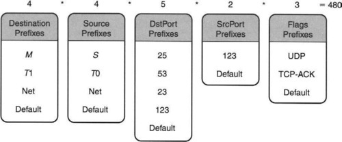
12.10 CROSS-PRODUCTING
This section describes a crude scheme called cross-producting [SVSW98]. In the next section, we describe a crucial refinement we call equivalenced cross-producting (but called RFC by the authors [GM99b]) that makes cross-producting more feasible. The top of each column in Figure 12.11 indicates the number of elements in the column. Consider a 5-tuple, formed by taking one value from each column. Call this a cross product. Altogether, there are 4 * 4 * 5 * 2 * 3 = 480 possible cross products. Some sample cross products are shown in Figure 12.13. Considering the destination field to be most significant and the flags field to be least significant, and pretending that values increase down a column, cross products can be ordered from the smallest to the largest, as in any number system.
A key insight into the utility of cross products is as follows.
Given a packet header H, if the longest-matching-prefix operation for each field H[i] is concatenated to form a cross product C, then the least-cost rule matching H is identical to the least-cost rule matching C.
Suppose this were not true. Since each field in C is a prefix of the corresponding field in H, every rule that matches C also matches H. Thus the only case in which H has a different matching rule is if there is some rule R that matches H but not C. This implies that there is some field i such that R[i] is a prefix of H[i] but not of C[i], where C[i] is the contribution of field i to cross product C. But since C[i] is a prefix of H[i], this can happen only if R[i] is longer than C[i]. But that contradicts the fact that C[i] is the longest-matching prefix in column/field i.
Thus, the basic cross-producting algorithm [SVSW98] builds a table of all possible cross products and precomputes the least-cost rule matching each cross product. This is shown in Figure 12.13. Then, given a packet header, the search algorithm can determine the least-cost matching rule for the packet by performing K longest-matching-prefix operations, together with a single hash lookup of the cross-product table. In hardware, each of the K prefix lookups can be done in parallel.
Using our example, consider matching a packet with header (M, S, UDP, 53,57) in the database of Figure 12.3. The cross product obtained by performing best-matching prefixes on individual fields is (M, S, UDP, 53, default). It is easy to check that the precomputed rule for this cross product is Rule 2 — although Rules 3 and 8 also match the cross product, Rule 2 has the least cost.
The naive cross-producting algorithm suffers from a memory explosion problem: In the worst case, the cross-product table can have NK entries, where N is the number of rules and K is the number of fields. Thus, even for moderate values, say, N = 100 and K = 5, the table size can reach 1010, which is prohibitively large.
One idea to reduce memory is to build the cross products on demand (P2b, lazy evaluation) [SVSW98]: Instead of building the complete cross-product table at the start, the algorithm incrementally adds entries to the table. The prefix tables for each field are built as before, but the cross-product table is initially empty. When a packet header H arrives, the search algorithm performs a longest-matching prefixes on the individual fields to compute a cross-product term C.
If the cross-product table has an entry for C, then of course the associated rule is returned. However, if there is no entry for C in the cross-product table, the search algorithm finds the best-matching rule for C (possibly using a linear search of the database) and inserts that entry into the cross-product table. Of course, any subsequent packets with cross product C will yield fast lookups.
On-demand cross-producting can improve both the building time of the data structure and its storage cost. In fact, the algorithm can treat the cross-product table as a cache and remove all cross products that have not been used recently. Caching based on cross products can be more effective than full header caching because a single cross product can represent multiple headers (see Exercises). However, a more radical improvement of cross-producting comes from the next idea, which essentially aggregates cross products into a much smaller number of equivalence classes.
12.11 EQUIVALENCED CROSS-PRODUCTING
Gupta and McKeown [GM99b] have invented a scheme called recursive flow classification (RFC), which is an improved form of cross-producting that significantly compresses the cross-product table, at a slight extra expense in search time. We prefer to call their scheme equivalenced cross-producting, for the following reason. The scheme works by building larger cross products from smaller cross products; the main idea is to place the smaller cross products into equivalence classes before combining them to form larger cross products. This equivalencing of partial cross products considerably reduces memory requirements, because seVeral original cross-product terms map into the same equivalence class.
Recall that in simple cross-producting when a header H arrives, the individual field matches are immediately concatenated to form a cross product that is then looked up in a cross-product table. By contrast, equivalenced cross-producting builds the final cross product in several pairwise combining steps instead of in one fell swoop.
For example, one could form the destination–source cross product and separately form the destination port–source port cross product. Then, a third step can be used to combine these two cross products into a cross product on the first four fields, say, C′. A fourth step is then needed to combine C′ with the protocol field to form the final cross product, C. The actual combining sequence is defined by a combining tree, which can be chosen to reduce overall memory.
Just forming the final cross product in several pairwise steps does not reduce memory below NK. What does reduce memory is the observation that when two partial cross products are combined, many of these pairs are equivalent: Geometrically, they correspond to the same region of space; algebraically, they have the same set of compatible rules.
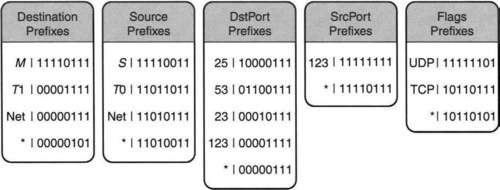
Thus the main trick is to give each class a class number and to form the larger cross products using the class numbers instead of the original matches. Since the algebraic view is easier for computation, we will describe an example of equivalencing using the first two columns of Figure 12.11 under the algebraic view.
Figure 12.14 shows the partial cross products formed by only the destination and source columns in Figure 12.11. For each pair (e.g., M,S) we compute the set of rules that are compatible with such a pair of matches exactly, as in the bit vector linear search scheme. In fact, we can find the bit vector of any pair, such as M, S, by taking the intersection of the rule bitmaps for M and S in Figure 12.12. Thus from Figure 12.12, since the rule bitmap for M is 11110111 and the bitmap for S is 11110011, the intersection bitmap for M,S is 11110011, as shown in Figure 12.14.
Doing this for each possible pair, we soon see that several bitmaps repeat themselves. For example, M, T0, and M, * (second and fourth entries in Figure 12.14) have the same bitmap. Two rules that have the same bitmap are assigned to the same equivalence class, and each class is given a class number. Thus in Figure 12.14, the classes are numbered starting with 1; the table-building algorithm increments the class number whenever it encounters a new bitmap. Thus, there are only eight distinct class numbers, compared to 16 possible cross products, because there are only eight distinct bitmaps.
Now assume we combine the two port columns to form six classes from 10 possible cross products. When we combine the port pairs with the destination–source pairs, we combine all possible combinations of the destination–source and port pair class numbers and not the original field matches. Thus after combining all four columns we get 6 * 8 = 48 cross products. Note that in Figure 12.11, naive cross-producting will form 4 * 4 * 5 * 2 = 160 cross products from the first four columns. Thus we have saved a factor of nearly 3 in memory.
Of course, we do not stop here. After combining the destination–source and port pair class numbers we equivalence them again using the same technique. When combining class number C with class number C′, the bitmap for C, C′ is the intersection of the bitmaps for C and C′. Once again pairs with identical bitmaps are equivalenced into groups. After this is done, the final cross product is formed by combining the classes corresponding to the first four columns with the matches in the fifth column.
Our example combined fields 1 and 2, then fields 3 and 4, and then the first four and finally combined in the fifth (Figure 12.15). Clearly, other pairings are possible, as defined by a binary tree with the fields as nodes and edges representing pairwise combining steps. One could choose the optimal combining tree to reduce memory.
The search process is similar to cross-producting, except the cross products are calculated pairwise (just as they are built) using the same tree. Each pairwise combining uses the two class numbers as input into a table that outputs the class number of the combination. Finally, the class number of the root of the tree is looked up in a table to yield the best-matching rule. Since each class has the same set of matching rules, it is easy to precompute the lowest-cost matching rule for the final classes. Note that the search process does not need to access the rule bitmaps, as is needed for the bit vector linear search scheme. The bitmaps are used only to build the structure.
Clearly, each pairwise combining step can take O(N2) memory because there can be N distinct field values in each field. However, the total memory falls very short of the NK worst-case memory for real rule databases. To see why this might be the case, we return to the geometric view.
Using a survey of 8000 rule databases, Gupta and McKeown [GM99b] observe that all databases studied have only O(N) classification regions, instead of the NK worst-case number of classification regions. It is not hard to see that when the number of classification regions is NK, then the number of cross products in the equivalenced scheme and in the naive scheme is also NK.
But when the number of classification regions is linear, equivalenced cross-producting can do better. However, it is possible to construct counterexamples where the number of classification regions is linear but equivalenced cross-producting takes exponential memory. Despite such potentially pathological cases, the performance of RFC can be summarized as follows.
Assumption: There is a series of subspaces of the complete rule space (as embodied by nodes in the combining tree) that all have a linear number of classification regions. Note that this is stronger than O4 and even O5. For example, if we combine two fields i and j first, we require that this intermediate two-dimensional subspace have a linear number of regions.
Performance: The memory required is O(N2) * T, where T is the number of nodes in the combining tree. The sequential performance (in terms of time) is O(T) memory accesses, but the time required in a parallel implementation can be O(1) because the tree can be pipelined. Note that the O(N2) memory is still very large in practice and would preclude the use of SRAM-based solutions.
12.12 DECISION TREE APPROACHES
This chapter ends with a description of a very simple scheme that performs well in practice, better even than RFC and comparable to or better than the extended grid of tries. This scheme was introduced by Woo [Woo00]. A similar idea, with range tests replacing bit tests, was independently described by Gupta and McKeown [GM99a].
The basic idea is extremely close to the simple set-pruning tries described in Section 12.5.1, with the addition of some important degrees of freedom. Recall that set-pruning tries work one field at a time; thus in Figure 12.8, the algorithm tests all the bits for the destination address before testing all the bits for the source address. The extension to multiple fields in Decasper et al. [DDPP98] similarly tests all the bits of one field before moving on to another field. The set-pruning trie can be seen as an instance of a general decision tree.
Clearly, an obvious degree of freedom (P13) not considered in set-pruning tries is to arbitrarily interleave the bit tests for all fields. Thus the root of the trie could test for (say) bit 15 of the source field; if the bit is 0, this could lead to a node that tests for, say, bit 22 of the port number field. Clearly, there is an exponential number of such decision trees. The schemes in Woo [Woo00] and Gupta and McKeown [GM99a] build the final decision tree using local optimization decisions at each node to choose the next bit to test. A simple criterion used in Gupta and McKeown [GM99a] is to balance storage and time.
A second important degree of freedom considered in Woo [Woo00] is to use multiple decision trees. For example, for examples such as Figure 12.6, it may help to place all the rules with wildcards in the source field in one tree and the remainder in a second tree. While this can increase overall search time, it can greatly reduce storage.
A third degree of freedom exploited in both Woo [Woo00] and Gupta and McKeown [GM99a] is to allow a small amount of linear searching after traversing the decision tree. This is similar to the common strategy of using an insert. Consider a decision tree with 10,000 leaves where each leaf is associated with one of four rules. While it may be possible to distinguish these four rules by lengthening the decision tree in height, this lengthened decision tree could add 40,000 extra nodes of storage.
Thus, in balancing storage with time, it may be better to settle for a small amount of linear searching (e.g., among one of four possible rules) at the end of tree search. Intuitively, this can help because the storage of a tree can increase exponentially with its height. Reducing the height by employing some linear search can greatly reduce storage.
The hierarchical cuttings (HiCuts) scheme described in Gupta and McKeown [GM99a] is similar in spirit to that in Woo [Woo00] but uses range checks instead of bit tests at each node of the decision tree. Range checks are slightly more general than bit tests because a range check such as 10 < D < 35 for a destination address D cannot be emulated by a bit test. A range test (cut) can be viewed geometrically in two dimensions as a line in either dimension that splits the space into half; in general, each range cut is a hyperplane.
In what follows, we describe HiCuts in more detail using an example. The HiCuts local optimization criterion works well when tested on real core router classifiers.
Figure 12.16 shows a fragment of a HiCuts decision tree on the database of Figure 12.3. The nodes contain range comparisons on values of any specified fields, and the edges are labeled True or False. Thus the root node tests whether the destination port field is less than 50. The fragment follows the case only when this test is false. Notice in Figure 12.3 that this branch eliminates R1 (i.e., Rule 1) and R4, because these rules contain port numbers 25 and 23, respectively.
The next test checks whether the source address is equal to that of the secondary name server S in Figure 12.3. If this test evaluates to true, then R5 is eliminated (because it contains T0,), and so is R6 (because it contains Net and because S does not belong to the internal prefix Net). This leads to a second test on the destination port field. If the value is not 53, the only possible rules that can match are R7 and R8.
Thus on a packet header in which the destination port is 123 and the source is S, the search algorithm takes the right branch at the root, the left branch at the next node, and a right branch at the final node. At this point the packet header is compared to rules R7 and R8 using linear search. Note that, unlike set pruning trees, the HiCuts decision tree of Figure 12.16 uses ranges, interleaves the range checks between the destination port and source fields, and uses linear searching.
Of course, the real trick is to find a way to build an efficient decision tree that minimizes the worst-case height and yet has reasonable storage. Rather than consider the general optimization problem, which is NP-complete, HiCuts [GM99a] uses a more restricted heuristic based on the repeated application of the following greedy strategy.
• Pick a field: The HiCuts paper suggests first picking a field to cut on at each stage based on the number of distinct field values in that field. For example, in Figure 12.16, this heuristic would pick the destination port field.
• Pick the number of cuts: For each field, rather than just pick one range check as in Figure 12.16, one can pick k ranges or cuts. Of course, these can be implemented as separate range checks, as in Figure 12.16. To choose k, the algorithm suggested in Gupta and McKeown [GM99b] is to keep doubling k and to stop when the storage caused by the k cuts exceeds a prespecified threshold.
Several details are needed to actually implement this somewhat general framework. Assuming the cuts or ranges are equally spaced, the storage cost of k cuts on a field is estimated by counting the sum of the rules assigned to each of the k cuts. Clearly, cuts that cause rule replication will have a large storage estimate. The threshold that defines acceptable storage is a constant (called spfac, for space factor) times the number of rules at the node. The intent is to keep the storage linear in the number of rules up to a tunable constant factor.
Finally, the process stops when all decision tree leaves have no more than binth (bin threshold) rules, binth controls the amount of linear searching at the end of tree search.
The HiCuts paper [GM99a] mentions the use of the DAG optimization. A more novel optimization, described in Woo [WooOO] and Gupta and McKeown [GM99a], is to eliminate a rule, R, that completely overlaps another rule, R′, at a node but has higher cost. There are also several further degrees of freedom (P13) left unexplored in Gupta and McKeown [GM99a] and Woo [Woo00]: unequal-size cuts at each node, more sophisticated strategies that pick more than field at a time, and linear searching at nodes other than the leaves.
A more recent paper [BSV03] takes the decision tree approach a step further by allowing the use of several cuts in a single step via multidimensional array indexing. Because each cut is now a general hypercube, the scheme is called HyperCuts. HyperCuts appears to work significantly faster than HiCuts on many real databases [BSV03].
In conclusion, the decision tree approach described by Woo [Woo00], Gupta and McKeown [GM99a], and Singh et al. [BSV03] is best viewed as a framework which encompasses a number of potential algorithms. However, experimental evidence [BSV03] shows that this approach works well in practice except on databases that contain a large number of wildcards in one or more fields. The performance of this scheme can be summarized as follows.
Assumption: The scheme assumes there is a sufficient number of distinct fields to make reasonable cuts without much storage replication. This rather general observation needs to be sharpened.
Performance: The memory required can be kept to roughly linear in the number of rules using the HiCuts heuristics. The tree can be of relatively small height if it is reasonably balanced. Search can easily be pipelined to allow O(1) lookup times. Finally, update can be slow if sophisticated heuristics are used to build the decision tree.
12.13 CONCLUSIONS
This chapter describes several algorithms for packet classification at gigabit speeds. The grid of tries provides a two-dimensional classification algorithm that is fast and scalable. All the remaining schemes require exploiting some assumption about real rule databases to avoid the geometric lower bound. While much progress has been made, it is important to reduce the number of such assumptions required for classification and to validate these assumptions extensively.
At the time of writing, decision tree approaches [Woo00, GM99a, SBV04] and the extended grid of tries method [BSV03] appeared to be the most attractive algorithmic schemes. While the latter depends on each packet’s matching only a small number of source–destination prefixes, it is still difficult to characterize what assumptions or parameters influence the performance of decision tree approaches.
Of the other general schemes, the bit vector scheme is suitable for hardware implementation for a modest number of rules (say, up to 10,000). Equivalenced cross-producting seems to scale to roughly the same number of rules as the Lucent scheme but perhaps can be improved to lower its memory consumption.
The author and his students have placed code for many of the algorithms described in this chapter on a publicly available Web site [SBV04]. Packet classification has stagnated because of the lack of standard comparisons and freely available code. Readers are encouraged to experiment with and contribute to this code base.
Although the schemes described in this chapter require some algorithmic thinking, they make heavy use of the other principles we have stressed. The two-dimensional scheme makes heavy use of precomputation; the Lucent scheme uses memory locality to turn what is essentially linear search into a fast scheme for moderate rule sizes; all the other schemes rely on some expected-case assumption about the structure of rules, such as the lack of general ranges and the small number of classification regions. Figure 12.1 summarizes the schemes and the principles used in them.
Because best-matching prefix is a special case of lowest-cost matching rule, it is not surprising that rule search schemes are generalizations of prefix search schemes. Thus, the grid of tries and set-pruning tries generalize trie schemes for prefix matching. Multidimensional range-matching schemes generalize prefix-matching schemes based on range matching. Tuple search generalizes binary search on hash tables. While cross-producting is not a generalization of an existing prefix-matching scheme, it can be specialized for prefix lookups as well.
The high-level message of this chapter is as follows. Applications such as QoS routing, firewalls, virtual private networks, and DiffServ will require a more flexible form of forwarding based on multiple header fields. The techniques in this chapter indicate that such forwarding flexibility can go together with high performance using algorithmic solutions without relying on ternary CAMs.
Returning to the quote at the start of this chapter, it should be easy to see how packet classification gets its name if the word definition is replaced with rule. Notice that classification in the sciences also encompasses overlapping definitions: Men belong to both the mammal and Homo sapiens categories. However, it is hard to imagine a biological analog of the concept of a lowest-cost matching rule, or the requirement to classify species several million times a second!
12.14 EXERCISES
1. Range to Prefix Mappings: CAMs require the use of prefix ranges, but many rules use general ranges. Describe an algorithm that converts an arbitrary range on, say, 16-bit port number fields to a logarithmic number of prefix ranges. Describe the prefix ranges produced by the arbitrary but common range of greater than 1024. Given a rule R with arbitrary range specifications on port numbers, what is the worst-case number of CAM entries required to represent R? Solutions to this problem are discussed in Refs. SVSW98 and SSV99.
2. Worst-Case Storage for Set-Pruning Tries: Generalize the example of Figure 12.6 to K fields to show that storage in set-pruning-trie approaches can be as bad as O(Nk/k).
3. Improvements to the Grid of Tries: In the grid of tries, the only role played by the destination trie is in determining the longest-matching destination prefix. Show how to use other lookup techniques to obtain a total search time of (log W + W) for destination–source rules instead of 2W.
4. Aggregate Bit Vector Search: Use 3-bit summaries in Figure 12.12 and determine the improvement in the worst-case time by adding summaries, and compare it to the increase in storage for using summaries. Details of the algorithm, if needed, can be found in Baboescu and Varghese [BV01].
5. Aggregate Bit Vector Storage: The use of summary bits appears to increase storage. Show, however, a simple modification in which the use of aggregates can reduce storage if the bit vectors contain large strings of zeroes. Describe the modifications to the search process to achieve this compression. Does it slow down search?
6. On-Demand Cross-Producting: Consider the database of Figure 12.3, and imagine a series of Web accesses from an internal site to the external network. Suppose the external destinations accessed are D1,…, DM. How many cache terms will these headers produce in the case of full header caching versus on-demand cross-producting?
7. Equivalenced Cross-Producting: Why do the fifth and eighth entries in Figure 12.14 have the same bitmaps? Check your answer two ways, first by intersecting the corresponding bitmaps for the two fields from Figure 12.12 and then by arguing directly that they match the same set of rules.
8. Combining Trees for RFC: The equivalenced cross-producting idea in RFC leaves unspecified how to choose a combining tree. One technique is to compute all possible combining trees and then to pick the tree with the smallest storage. Describe an algorithm based on dynamic programming to find the optimal tree. Compare the running times of the two algorithms.
9. Reducing Rule Databases Using Redundancy: If a smaller prefix has the same next hop as a longer prefix, the longer prefix can be removed from an IP lookup table. Find similar techniques to spot redundancies in classifiers. Compare your ideas with the techniques described in Gupta and McKeown [GM99b]. Note that as in the case of IP lookups, such techniques to remove redundancy are orthogonal to the classification scheme chosen and can be implemented in a separate preprocessing step.
10. Generalizing Linear Searching in HiCuts: In HiCuts, all the linear lists are at the leaves. However, a rule with all wildcarded entries will be replicated at all leaves. This suggests that such rules be placed once in a linear list at the root of the HiCuts tree. Generalizing, one could place linear lists at any node to reduce storage. Describe a bottom-up algorithm that starts with the base HiCuts decision tree and then hoists rules to nodes higher up in the tree to reduce storage. Try to do so with minimal impact on the search time.