
Measuring Network Traffic
Not everything that is counted counts, and not everything that counts can be counted.
— ALBERT EINSTEIN
Every graduate with a business degree knows that the task of optimizing an organization or process begins with measurement. Once the bottlenecks in a supply chain are identified and the major cost factors are outlined, improvements can be targeted. The situation is no different in computer networks. For example, in service provider networks, packet counting and logging provide powerful tools for the following.
Capacity Planning: Internet service providers (ISPs) need to determine the traffic matrix, or the traffic between all source and destination subnets they connect. This knowledge can be used on short time scales (say, hours) to perform traffic engineering by reconfiguring optical switches; it can also be used on longer time scales (say, months) to upgrade link capacity.
Accounting: Internet service providers implement complex service level agreements (SLAs) with customers and peers. Simple accounting arrangements based on overall traffic can easily be monitored by a single counter; however, more sophisticated agreements based on traffic type require a counter per traffic type. Packet counters can also be used to decide peering relationships. Suppose ISP A is currently sending packets to ISP C via ISP B and is considering directly connecting (peering) with B; a rational way for A to decide is to count the traffic destined to prefixes corresponding to B.
Traffic Analysis: Many network managers monitor the relative ratio of one packet type to another. For example, a spike in peer-to-peer traffic, such as to Kazaa, may require rate limiting. A spike in ICMP messages may indicate a Smurf attack.
Once causes — such as links that are unstable or have excessive traffic — are identified, network operators can take action by a variety of means. Thus measurement is crucial not just to characterize the network but to better engineer its behavior.
There are several control mechanisms that network operators currently have at their disposal. For example, operators can tweak Open Shortest Path First (OSPF) link weights and BGP policy to spread load, can set up circuit-switched paths to avoid hot spots, and can simply buy new equipment. This chapter focuses only on network changes that address the measurement problem — i.e., changes that make a network more observable. However, we recognize that making a network more controllable, for instance, by adding more tuning knobs, is an equally important problem we do not address here.
Despite its importance, traffic measurement, at first glance, does not appear to offer any great challenges or have much intellectual appeal. As with mopping a floor or washing dishes, traffic measurement appears to be a necessary but mundane chore.
The goal of this chapter is to argue the contrary: that measurement at high speeds is difficult because of resource limitations and lack of built-in support; that the problems will only grow worse as ISPs abandon their current generation of links for even faster ones; and that algorithmics can provide exciting alternatives to the measurement quandary by focusing on how measurements will ultimately be used. To develop this theme, it is worth understanding right away why the general problem of measurement is hard and why even the specific problem of packet counting can be difficult.
This chapter is organized as follows. Section 16.1 describes the challenges involved in measurement. Section 16.2 shows how to reduce the required width of an SRAM counter using a DRAM backing-store. Section 16.3 details a different technique for reducing counter widths by using randomized counting, which trades accuracy for counter width. Section 16.4 presents a different approach to reducing the number of counters required (as opposed to the width) by keeping track of counters only above a threshold. Section 16.5 shows how to reduce the number of counters even further for some applications by counting only the number of distinct flows.
Techniques in prior sections require computation on every packet. Section 16.6 takes a different tack by describing the sampled NetFlow technique for reducing packet processing; in NetFlow only a random subset of packets is processed to produce either a log or an aggregated set of counters. Section 16.7 shows how to reduce the overhead of shipping NetFlow records to managers. Section 16.8 explains how to replace the independent sampling method of Net-Flow with a consistent sampling technique in all routers that allow packet trajectories to be traced.
The last three sections of the chapter move to a higher-level view of measurement. In Section 16.9 we describe a solution to the accounting problem. This problem is of great interest to ISPs, and the solution method is in the best tradition of the systems approach advocated throughout this book. In Section 16.10 we describe a solution to the traffic matrix problem using the same concerted systems approach. Section 16.11 presents a very different approach to measurement called passive measurement, that treats the network as a black box. It includes an example of the use of passive measurement to compute the loss rate to a Web server.
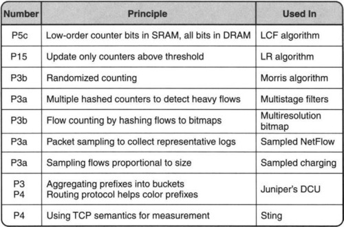
The implementation techniques for the measurement primitives described in this chapter (and the corresponding principles used) are summarized in Figure 16.1.
16.1 WHY MEASUREMENT IS HARD
Unlike the telephone network, where observability and controllability were built into the design, the very simplicity of the successful Internet service model has made it difficult to observe [DG00]. In particular, there appears to be a great semantic distance between what users (e.g., ISPs) want to know and what the network provides. In this tussle [CWSB02] between user needs and the data generated by the network, users respond by distorting [CWSB02] existing network features to obtain desired data.
For example, Traceroute uses the TTL field in an admittedly clever but distorted way, and the Path MTU discovery mechanism is similar. Tools like Sting [Sav99] use TCP in even more baroque fashion to yield end-to-end measures. Even tools that make more conventional use of network features to populate traffic matrices (e.g., Refs. FGeaOO and ZRDG03) bridge the semantic gap by correlating vast amounts of spatially separated data and possibly inconsistent configuration information. All this is clever, but it may not be engineering.1 Perhaps much of this complexity could be removed by providing measurement features directly in the network.
One of the fundamental tools of measurement is counting: counting the number of packets or events of a given type. It is instructive to realize that even packet counting is hard as we show next.
16.1.1 Why Counting Is Hard
Legacy routers provide only per-interface counters that can be read by the management protocol SNMP. Such counters count only the aggregate of all counters going on an interface and make it difficult to estimate traffic AS-AS matrices that are needed for traffic engineering. They can also be used only for crude forms of accounting, as opposed to more sophisticated forms of accounting that count by traffic type (e.g., real-time traffic may be charged higher) and destination (some destinations may be routed through a more expensive upstream provider).
Thus vendors have introduced filter-based accounting, where customers can count traffic that matches a rule specifying a predicate on packet header values. Similarly, Cisco provides NetFlow-based accounting [Net], where sampled packets can be logged for later analysis, and 5-tuples can be aggregated and counted on the router. Cisco also provides Express Forwarding commands, which allow per-prefix counters [Cis].
Per-interface counters can easily be implemented because there are only a few counters per interface, which can be stored in chip registers. However, doing filter-based or per-prefix counters is more challenging because of the following.
• Many counters: Given that even current routers support 500,000 prefixes and that future routers may have a million prefixes, a router potentially needs to support millions of real-time counters.
• Multiple counters per packet: A single packet may result in updating more than one counter, such as a flow counter and a per-prefix counter.
• High speeds: Line rates have been increasing from OC-192 (10 Gbps) to OC-768 (40 Gbps). Thus each counter matched by a packet must be read and written in the time taken to receive a packet at line speeds.
• Large widths: As line speeds get higher, even 32-bit counters overflow quickly. To prevent the overhead of frequent polling, most vendors now provide 64-bit counters.
One million counters of 64 bits each requires a total of 64 Mbits of memory; while two counters of 64 bits each every 8 nec requires 16 Gbps of memory bandwidth. The memory bandwidth needs require the use of SRAM, but the large amount of memory needed makes SRAM of this size too expensive. Thus maintaining counters or packet logs at wire speeds is as challenging as other packet-processing tasks, such as classification and scheduling; it is the focus of much of this chapter.
In summary, this section argues that: (i) packet counters and logs are important for network monitoring and analysis; (ii) naive implementations of packet counting and logs require potentially infeasible amounts of fast memory. The remainder of this chapter describes the use of algorithmics to reduce the amount of fast memory and processing needed to implement counters and logs.
16.2 REDUCING SRAM WIDTH USING DRAM BACKING STORE
The next few sections ignore the general measurement problem and concentrate on the specific problem of packet counting. The simplest way to implement packet counting is shown in Figure 16.2. One SRAM location is used for each of, say, 1 million 64-bit counters. When a packet arrives, the corresponding flow counter (say, based on destination) is incremented.

Given that such large amounts of SRAM are expensive and infeasible, is it required? If a packet arrives, say, every 8 nsec, some SRAM counter must be accessed — as opposed to, say, 40-nsec DRAM. However, intuitively keeping a full 64-bit SRAM location is obvious waste (P1).
Instead, the best hardware features of DRAM and SRAM can be combined (P5c). DRAM is at least four times cheaper and often as much as 10 times cheaper, depending on market conditions. On the other hand, DRAM is slow. This is exactly analogous to the memory hierarchy in a computer. The analogy suggests that DRAM and SRAM can be combined to provide a solution that is both cheap and fast.
Observe that if the router keeps a 64-bit DRAM backing location for each counter and a much smaller width (say, 12 bits) for each SRAM counter, then the counter system will be accurate as long as every SRAM counter is backed up to DRAM before the smaller SRAM counter overflows. This scheme is depicted in Figure 16.3. What is missing, however, is a good algorithm (P15) for deciding when and how to back up SRAM counters.

Assume that the chip maintaining counters is allowed to dump some SRAM counter to DRAM every b SRAM accesses, b is chosen to be large enough that b SRAM access times correspond to 1 DRAM access time. In terms of the smallest SRAM width required, Shah et al. [SIPM02] show that the optimal counter-management algorithm is to dump the largest SRAM counter. With this strategy Shah et al. [SIPM02] show that the SRAM counter width c can be significantly smaller than M, the width of a DRAM counter.
More precisely, they show that ![]() , where N is the total number of counters. Note that this means that the SRAM counter width grows approximately as log log bN, since b/b – 1 can be ignored for large b. For example, with three 64-bit counters every 8 nsec (OC-768) for N equal to a million requires only 8 Mbit of 2.5 μsec SRAM with 51.2 μsec DRAM. Note that in this case the value of b is 51.2/2.5 ≈ 21.
, where N is the total number of counters. Note that this means that the SRAM counter width grows approximately as log log bN, since b/b – 1 can be ignored for large b. For example, with three 64-bit counters every 8 nsec (OC-768) for N equal to a million requires only 8 Mbit of 2.5 μsec SRAM with 51.2 μsec DRAM. Note that in this case the value of b is 51.2/2.5 ≈ 21.
The bottom line is that the naive method would have required 192 Mbit of SRAM compared to 8 Mbit, a factor of 24 savings in expensive SRAM. Overall, this provides roughly a factor of 4 savings in cost, assuming DRAM is four times cheaper than SRAM.
But this begs the question. How does the chip processing counters find the the largest counter? Bhagwan and Lin [BL00] describe an implementation of a pipelined heap structure that can determine the largest value at a fairly high expense in hardware complexity and space. Their heap structure requires pointers of size log2 N for each counter just to identify the counter to be evicted. Unfortunately, log2 N additional bits per counter can be large (20 for N = 1 million) and can defeat the overall goal, which was to reduce the required SRAM bits from 64 to say 10.
The need for a pointer per heap value seems hard to avoid. This is because the counters must be in a fixed place to be updated when packets arrive, but values in a heap must keep moving to maintain the heap property. On the other hand, when the largest value arrives at the top of the heap, one has to correlate it to the counter index in order to reset the appropriate counter and to banish its contents to DRAM. Notice also that all values in the heap, including pointers and values, must be in SRAM for speed.
The following LR algorithm [RV03] simplifies the largest count first (LCF) algorithm of Shah et al. [SIPM02] and is easier to implement. Let j be the index of the counter with the largest value among the counters incremented in the last cycle of b updates to SRAM. Ties may be broken arbitrarily. If cj ≥ b, the algorithm updates counter cj to DRAM. If cj < b, the algorithm updates any counter with value at least b to DRAM. If no such counter exists, LR(T) updates counter Cj to DRAM.
It can be shown that LR [RV03] is also optimal and produces SRAM counter width c, which is equal to that of LCF. The maintaining of all counters above the threshold b can be done using a size-N bitmap in which a 1 implies that the corresponding position has a counter no less than b.
This leaf structure can be augmented with a simple tree that maintains the position of the first 1 (see Exercises). The tree can be easily pipelined for speed, and only roughly 2 bits per counter are required for this additional data structure; thus c is increased from its optimal value, say, x to x + 2, a reasonable cost.
Thus the final LR algorithm is a better algorithm (P15) and one that is easier to implement, provides a new data structure to efficiently find the first bit set in a bitmap (P15), and adds pipelining hardware (P5) to gain speed.
The overall approach could be considered superficially similar to the usual use of the memory hierarchy, in which a faster memory acts as a cache for a slower memory. However, unlike a conventional cache this design ensures worst-case performance and not expected case performance. The goals of the two algorithms are also different: Counter management stores an entry for all items but seeks to reduce the width of cache entries, while standard caching stores full widths for only some frequent items.
16.3 REDUCING COUNTER WIDTH USING RANDOMIZED COUNTING
The DRAM backing-store approach trades off reduced counter widths for more processing and complexity. A second approach is to trade accuracy and certainty (P3a, b) for reduced counter widths. For many applications described earlier, approximate counters may suffice.
The basic idea is as follows. If we increment a b-bit counter only with probability 1/c, then when the counter saturates, the expected number of counted events is 2b · c. Thus a b-bit randomized counter can count c times more events than a deterministic version. But once the notion of approximate counting is accepted, it is possible to do better.
Notice that in the basic idea, the standard deviation (i.e., the expected value of the counter error) is a few c’s, which is small at counter values >> c. R. Morris’s idea for randomized counting is to notice that for higher counter values, one can tolerate higher absolute values of the error. For example, if the standard deviation is equal to the counter, the real value is likely to be within half to twice the value determined by the counter. Allowing the error to scale with counter values in turn allows a smaller counter width.
To achieve this, Morris’s scheme increments a counter with nonconstant probability that depends on counter value, so expected error scales with counter size. Specifically, the algorithm increments a counter with probability 1/2x, where x is the value of the counter. At the end, a counter value of x represents an expected value of 2x. Thus the number of bits required for such a counter is log log Max, where Max is the maximum value required for the counter.
While this is an interesting scheme, its high standard deviation and the need to pick accurate small numbers, especially for high values of the counter, are clear disadvantages. Randomized counting is an example of using P3b, trading accuracy for storage (and time).
16.4 REDUCING COUNTERS USING THRESHOLD AGGREGATION
The last two schemes reduce the width of the SRAM counter table shown in Figure 16.2. The next two approaches reduce the height of the SRAM counter table. They rely on the quote from Einstein (which opened the chapter) that not all the information in the final counter table may be useful to an application, at least for some applications. Effectively, by relaxing the specification (P3), the number of counters that need to be maintained can be reduced.
One simple way to compress the counter table is shown in Figure 16.4. The idea is to pick a threshold, say, 0.1% of the traffic, that can possibly be sent in the measurement interval and to keep counters only for such “large” flows. Since, by definition, there can be at most 1000 such flows, the final table reduces to 1000 flow ID, counter pairs, which can be indexed using a CAM. Note that small CAMs are perfectly feasible at high speed.

This form of compression is reasonable for applications that only want counters above a threshold. For example, just as most cell phone plans charge a fixed price up to a threshold and a usage-based fee beyond the threshold, a router may only wish to keep track of the traffic sent by large flows. All other flows are charged a fixed price. Similarly, ISPs wishing to reroute traffic hot spots or detect attacks are only interested in large, “elephant” flows and not the “mice.”
However, this idea gives rise to a technical problem. How can a chip detect the elephants above the threshold without keeping track of all flows? The simplest approach would be to keep a counter for all flows, as in Figure 16.2, in order to determine which flows are above the threshold. However, doing so does not save any memory.
A trick [EV02] to directly compute the elephants together with the traffic sent by each elephant is shown in Figure 16.5. The building blocks are hash stages that operate in parallel. First, consider how the filter operates if it had only one stage. A stage is a table of counters indexed by a hash function computed on a packet flow ID; all counters in the table are initialized to 0 at the start of a measurement interval.

When a packet comes in, a hash on its flow ID is computed and the size of the packet is added to the corresponding counter. Since all packets belonging to the same flow hash to the same counter, if a flow F sends more than threshold T, F’s counter will exceed the threshold. If we add to the flow memory all packets that hash to counters of T or more, we are guaranteed to identify all the large flows (no false negatives).
Unfortunately, since the number of counters we can afford is significantly smaller than the number of flows, many flows will map to the same counter. This can cause false positives in two ways: first, small flows can map to counters that hold large flows and get added to flow memory; second, several small flows can hash to the same counter and add up to a number larger than the threshold.
To reduce this large number of false positives, the algorithm uses multiple stages. Each stage (Figure 16.5) uses an independent hash function. Only the packets that map to counters of T or more at all stages get added to the flow memory. For example, in Figure 16.5, if a packet with a flow ID F arrives that hashes to counters 3, 1, and 7, respectively, at the three stages, F will pass the filter (counters that are over the threshold are shown darkened).
On the other hand, a flow G that hashes to counters 7,5, and 4 will not pass the filter because the second-stage counter is not over the threshold. Effectively, the multiple stages attenuate the probability of false positives exponentially in the number of stages. This is shown by the following simple analysis.
Assume a 100-MB/sec link, with 100,000 flows. We want to identify the flows above 1% of the link during a 1-second measurement interval. Assume each stage has 1000 buckets and a threshold of 1 MB. Let’s see what the probability is for a flow sending 100 KB to pass the filter. For this flow to pass one stage, the other flows need to add up to 1 MB – 100 KB = 900 KB.
There are at most 99,900/900 = 111 such buckets out of the 1000 at each stage. Therefore, the probability of passing one stage is at most 11.1%. With four independent stages, the probability that a small flow no larger than 100 KB passes all four stages is the product of the individual stage probabilities, which is at most 1.52 * 10−4.
Note the potential scalability of the scheme. If the number of flows increases to 1 million, we simply add a fifth hash stage to get the same effect. Thus to handle 100,000 flows requires roughly 4000 counters and a flow memory of approximately 100 memory locations; to handle 1 million flows requires roughly 5000 counters and the same size of flow memory. This is logarithmic scaling.
The number of memory accesses at packet arrival time performed by the filter is exactly one read and one write per stage. If the number of stages is small enough, this is affordable, even at high speeds, since the memory accesses can be performed in parallel, especially in a chip implementation. A simple optimization called conservative update (see Exercises) can improve the performance of multistage filtering even further. Multistage filters can be seen as an application of Principle P3a, trading certainty (allowing some false positives and false negatives) for time and storage.
16.5 REDUCING COUNTERS USING FLOW COUNTING
A second way to reduce the number of counters even further, beyond even threshold compression, is to realize that many applications do not even require identifying flows above a threshold. Some only need a count of the number of flows. For example, the Snort (www.snort.org) intrusion-detection tool detects port scans by counting all the distinct destinations sent to by a given source and alarming if this amount is over a threshold.
On the other hand, to detect a denial-of-service attack, one might want to count the number of sources sending to a destination, because many such attacks use multiple forged addresses. In both examples, it suffices to count flows, where a flow identifier is a destination (port scan) or a source (denial of service).
A naive method to count source–destination pairs would be to keep a counter together with a hash table (such as Figure 16.2 except without the counter) that stores all the distinct 64-bit source–destination address pairs seen thus far. When a packet arrives with source and destination addresses S, D, the algorithm searches the hash table for S, D; if there is no match, the counter is incremented and S, D is added to the hash table. Unfortunately, this solution takes too much memory.
An algorithm called probabilistic counting [FM85] can considerably reduce the memory needed by the naive solution, at the cost of some accuracy in counting flows. The intuition behind probabilistic counting is to compute a metric of how uncommon a certain pattern within a flow ID is. It then keeps track of the degree of “uncommonness” across all packets seen. If the algorithm sees very uncommon patterns, the algorithm concludes it saw a large number of flows.
More precisely, for each packet seen, the algorithm computes a hash function on the flow ID. It then counts the number of consecutive zeroes, starting from the least significant position of the hash result; this is the measure of uncommonness used. The algorithm keeps track of X, the largest number of consecutive zeroes seen (starting from the least significant position) in the hashed flow ID values of all packets seen so far.
At the end of the interval, the algorithm converts X, the largest number of trailing zeroes seen, into an estimate 2X for the number of flows. Intuitively, if the stream contains two distinct flows, on average one flow will have the least significant bit of its hashed value equal to zero; if the stream contains eight flows, on average one flow will have the last three bits of its hashed value equal to zero — and so on.
Note that hashing is essential for two reasons. First, implementing the algorithm directly on the sequence of flow IDs itself could make the algorithm susceptible to flow ID assignments where the traffic stream contains a flow ID F with many trailing zeroes. If F is in the traffic stream, then even if the stream has only a few flows, the algorithm without hashing will wrongly report a large number of flows. Notice that adding multiple copies of the same flow ID to the stream will not change the algorithm’s final result, because all copies hash to the same value.
A second reason for hashing is that accuracy can be boosted using multiple independent hash functions. The basic idea with one hash function can guarantee at most 50% accuracy. By using N independent hash functions in parallel to compute N separate estimates of X, probabilistic counting greatly reduces the error of its final estimate. It does so by keeping the average value of X (as a floating point number, not an integer) and then computing 2X. Better algorithms for networking purposes are described in Estan et al. [EVF02].
The bottom line is that a chip can count approximately the number of flows with small error but with much less memory than required to track all flows. The computation of each hash function can be done in parallel. Flow counting can be seen as an application of Principle P3b, trading accuracy in the estimate for low storage and time.
16.6 REDUCING PROCESSING USING SAMPLED NETFLOW
So far we have restricted ourselves to packet counting. However, several applications might require packet logs. Packet logs are useful for analysts to retrospectively analyze for patterns and attacks.
In networking, there are general-purpose traffic measurement systems, such as Cisco’s NetFlow [Net], that report per-flow records for very fine grained flows, where a flow is identified by a TCP or UDP connection. Unfortunately, the large amount of memory needed to store packet logs requires the use of DRAM to store the logs. Clearly, writing to DRAM on every packet arrival is infeasible for high speeds, just as it was for counter management.
Basic NetFlow has two problems.
1. Processing Overhead: Updating the DRAM slows down the forwarding rate.
2. Collection Overhead: The amount of data generated by NetFlow can overwhelm the collection server or its network connection. Feldman et al. [FGea00] report loss rates of up to 90% using basic NetFlow.
Thus, for example, Cisco recommends the use of sampling (see Figure 16.6) at speeds above OC-3: Only the sampled packets result in updates to the DRAM flow cache that keeps the per-flow state. For example, sampling 1 in 16 packets or 1 in 1000 packets is common. The advantage is that the DRAM must be written to at most 1 in, say, 16 packets, allowing the DRAM access time to be (say) 16 times slower than a packet arrival time. Sampling introduces considerable inaccuracy in the estimate; this is not a problem for measurements over long periods (errors average out) and if applications do not need exact data.

The data-collection overhead can be alleviated by having the router aggregate the log information into counters (e.g., by source and destination autonomous systems (AS) numbers) as directed by a manager. However, Fang and Peterson [FP99] show that even the number of aggregated flows is very large. For example, collecting packet headers for Code Red traffic on a class A network [Moo01] produced 0.5 GB per hour of compressed NetFlow data. Aggregation reduced this data only by a factor of 4.
Sampling is an example of using P3a, trading certainty for storage (and time), via a randomized pruning algorithm.
16.7 REDUCING REPORTING USING SAMPLED CHARGING
A technique called sampled charging [DLT01] can be used to reduce the collection overhead of NetFlow, at the cost of further errors. The idea is to start with a NetFlow log that is aggregated by TCP or UDP connections and to reduce the overhead of sending this data to a collection station. The goal is to reduce collection bandwidth and processing, as opposed to reducing the size of the router log.
The idea, shown in Figure 16.7, is at first glance similar to threshold compression, described in Section 16.4. The router reports only flows above a threshold to the collection station. The only additional twist is that the router also reports a flow with size s that is less than the threshold with probability proportional to s.
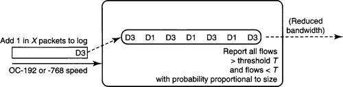
Thus the difference between this idea and simple threshold compression is that the final transmitted bandwidth is still small, but some attention is paid to flows below the threshold as well. Why might this be useful? Suppose all TCP individual connections in the aggregated log are small and below threshold but that 50% of the connections are from subnet A to subnet B.
If the router reported only the connections above threshold, the router would report no flows, because no individual TCP flow is large. Thus the collection agency would be unable to determine this unusual pattern in the destination and source addresses of the TCP connections. On the other hand, by reporting flows below threshold with a probability proportional to their size, on average half the flows the router will report will be from A to B. Thus the collection station can determine this unusual traffic pattern and take steps (e.g., increase bandwidth between these two) accordingly.
Thus the advantage of sampled charging over simple threshold compression is that it allows the manager to infer potentially interesting traffic patterns that are not decided in advance while still reducing the bandwidth sent to the collection node.
For example, sampled charging could also be used to detect an unusual number of packets sent by Napster using the same data sent to the collection station. Its disadvantage is that it still requires a large DRAM log. The large DRAM log scales poorly in size or accuracy as speeds increase.
On the other hand, threshold compression removes the need for the large DRAM log while directly identifying the large traffic flows. However, unless the manager knew in advance that he was interested in traffic between source and destination subnets, one cannot solve the earlier problem. For example, one cannot use a log that is threshold compressed with respect to TCP flows to infer that traffic between a pair of subnets is unusually large. Thus threshold compression has a more compact implementation but is less flexible than sample charging.
More formally, it can be shown that the multistage memory solution in Figure 16.5 requires ![]() memory, where M is the memory required by NetFlow or sampled charging for the same relative error. On the other hand, this solution requires more packet processing. Threshold compression is also less flexible than NetFlow and sampled charging in terms of being able to mine traffic patterns after the fact.
memory, where M is the memory required by NetFlow or sampled charging for the same relative error. On the other hand, this solution requires more packet processing. Threshold compression is also less flexible than NetFlow and sampled charging in terms of being able to mine traffic patterns after the fact.
Sampled charging is an example of using P3b, trading certainty for bandwidth (and time).
16.8 CORRELATING MEASUREMENTS USING TRAJECTORY SAMPLING
A final technique for router measurement is called trajectory sampling [DG00]. It is orthogonal to the last two techniques and can be combined with them. Recall that in sampled NetFlow and sampled charging, each router independently samples a packet. Thus the set of packets sampled at each router is different even when a set of routers sees the same stream of packets.
The main idea in trajectory sampling is to have routers in a path make correlated packet-sampling decisions using a common hash function. Figure 16.82 shows packets entering a router line card. The stream is “tapped” before it goes to the switch fabric. For every packet, a hash function h is used to decide whether the packet will be sampled by comparing the hashed value of the packet to a specified range. If the packet is sampled, a second hash function, g, on the packet is used to store a packet label in a log.

Trajectory sampling allows managers to correlate packets on different links. In order to ensure this, two more things are necessary. First, all routers must use the same values of g and h. Second, since packets can change header fields from router to router (e.g., TTL is decremented, data link header fields change), the hash functions are applied only to portions of the network packet that are invariant. This is achieved by computing the hash on header fields that do not change from hop to hop together with a few bytes of the packet payload.
A packet that is sampled at one router will be sampled at all routers in the packet’s trajectory or path. Thus a manager can use trajectory sampling to see path effects, such as packet looping, packet drops, and multiple shortest paths, that may not be possible to discern using ordinary sampled NetFlow.
In summary, the two differences between trajectory sampling and sampled NetFlow are:
(1) the use of a hash function instead of a random number to decide when to sample a packet;
(2) the use of a second hash function on invariant packet content to represent a packet header more compactly.
16.9 A CONCERTED APPROACH TO ACCOUNTING
In moving from efficient counter schemes to trajectory sampling, we moved from schemes that required only local support at each router to a scheme (i.e., trajectory sampling) that enlists the cooperation of multiple routers to extract more useful information. We now take this theme a step further by showing the power of concerted schemes that can involve all aspects of the network system (e.g., protocols, routers) at various time scales (e.g., route computation, forwarding). We provide two examples: an accounting example based on a scheme proposed by Juniper networks (described in this section) and the problem of traffic matrices (described in the next section).
The specific problem being addressed in this section is that of an ISP wishing to collect traffic statistics on traffic sent by a customer in order to charge the customer differently depending on the type of traffic and the destination of the traffic. Refer to Figure 16.9, which depicts a small ISP, Z, for the discussion that follows.
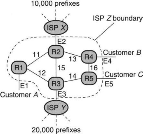
In the figure, assume that ISP Z wishes to bill Customer A at one rate for all traffic that exits via ISP X and at a different rate for all traffic that exits via ISP Y. One way to do this would be for router R1 to keep a separate counter for each prefix that represents traffic sent to that prefix. In the figure, R1 would have to keep at least 30,000 prefix counters. Not only does this make implementation more complex, but it is also unaligned with the user’s need, which will eventually aggregate the 30,000 prefixes into two tariff classes. Further, if routes change rapidly, the prefixes advertised by each ISP may change rapidly, requiring constant update of this mapping by the tool.
Instead, the Juniper DCU solution [Sem02] has two components.
1. Class Counters: Each forwarding table entry has a 16-bit class ID. Each bit in the class ID represents one of 16 classes. Thus if a packet matches prefix P with associated class ID C and C has bits set in bits 3, 6, and 9, then the counters corresponding to all three set bits are incremented. Thus there are only 16 classes supported, but a single packet can cause multiple class counters to be incremented. The solution aligns with hardware design realities because 16 counters per link is not much harder than one counter, and incrementing in parallel is easily feasible if the 16 counters are maintained on-chip in a forwarding ASIC. The solution also aligns with real user needs because it cheaply supports the use of up to 16 destination-sensitive3 counters.
2. Routing Support: To attack the problem of changing prefix routes (which would result in the tool’s having to constantly map each prefix into a different class), the DCU solution enlists the help of the routing protocol. The idea is that all prefixes advertised by ISP X are given a color (which can be controlled using a simple route policy filter), and prefixes advertised by ISP Y are given a different color. Thus when a router such as R1 gets a route advertisement for prefix P with color c, it automatically assigns prefix P to class c. This small change in the routing protocol greatly reduces the work of the tool.
Juniper also has other schemes [Sem02], including counters based on packet classifiers and counters based on MPLS tunnels. These are slightly more flexible than DCU accounting because they can take into account the source address of a packet in determining its class. But these other schemes do not have the administrative scalability of DCU accounting because they lack routing support.
The DCU accounting scheme is an example of P4, leveraging off existing system components, and P3, relaxing system requirements (e.g., only a small number of aggregate classes).
16.10 COMPUTING TRAFFIC MATRICES
While the DCU solution is useful only for accounting, a generalization of some of the essential ideas can help in solving the traffic matrix problem. This is a problem of great interest to many ISPs.
To define the traffic matrix problem, consider a network (e.g, Z in Figure 16.9) such as those used by ISPs Sprint and AT&T. The network can be modeled as a graph with links connecting router nodes. Some of the links from a router in ISP Z go to routers belonging to other ISPs (E2, E3) or customers (E1, E4, E5). Let us call such links external links. Although we have lumped them together in Figure 16.9, external links directed toward the ISP router are called input links, and external links directed away from an ISP router are called output links.
The traffic matrix of a network enumerates the amount of traffic that was sent (in some arbitrary period, say, a day) between every pair of input and output links of the network. For example, the traffic matrix could tell managers of ISP Z in Figure 16.9 that 60 Mbits of traffic entered during the day from Customer A, of which 20 Mbits exited on the peering link E2 to ISP X, and 40 Mbps left on link E5 to Customer B.
Network operators find traffic matrices (over various time scales ranging from hours to months) indispensable. They can be used to make more optimal routing decisions (working around suboptimal routing by changing OSPF weights or setting up MPLS tunnels), for knowing when to set up circuit-switched paths (avoiding hot spots), for network diagnosis (understanding causes of congestion), and for provisioning (knowing which links to upgrade on a longer time scale of months).
Unfortunately, existing legacy routers provide only a single aggregate counter (the SNMP link byte counter) of all traffic traversing a link, which aggregates traffic sent between all pairs of input and output links that traverse the link. Inferring the traffic matrix from such data is problematic because there are O(V2) possible traffic pairs in the matrix (where V is the number of external links), and many sparse networks may have only, say, O(V) links (and hence O(V) counters). Even after knowing how traffic is routed, one has O(V) equations for O(V2) variables, which makes deterministic inference (of all traffic pairs) impossible. This dilemma has led to two very different solution approaches. We now describe these two existing solutions and a proposed new approach.
16.10.1 Approach 1: Internet Tomography
This approach (see Refs. MTea02 and ZRDG03 for good reviews of past work) recognizes the impossibility of deterministic inference from SNMP counters cited earlier, and instead attempts statistical inference, with some probability of error. At the heart of the inference technique is some model of the underlying traffic distribution (e.g., Gaussian, gravity model) and some statistical (e.g., maximum likelihood) or optimization technique (e.g., quadratic programming [ZRDG03]4).
Early approaches based on Gaussian distributions did very poorly [MTea02], but a new approach based on gravity models does much better, at least on the AT&T backbone. The great advantage of tomography is that it works without retrofitting existing routers, and it is also clearly cheap to implement in routers. A possible disadvantage of this method is the potential errors in the method (off by as large as 20% in Zhang et al. [ZRDG03]), its sensitivity to routing errors (a single link failure can throw an estimate off by 50%), and its sensitivity to topology.
16.10.2 Approach 2: Per-Prefix Counters
Designers of modern routers have considered other systems solutions to the traffic matrix problem based on changes to router implementations and (sometimes) changes to routing protocols (see DCU scheme described earlier). For example, one solution being designed into some routers built at Cisco [Cis] and some start-ups is to use per-prefix counters. Recall that prefixes are used to aggregate route entries for many millions of Internet addresses into, say, 100,000–150,000 prefixes at the present time.
A router has a forwarding engine for each input line card that contains a copy of the forwarding prefix table. Suppose each prefix P has an associated counter that is incremented (by the number of bytes) for each packet entering the line card that matches P. Then by pooling the per-prefix counters kept at the routers corresponding to each input link, a tool can reconstruct the traffic matrix. To do so, the tool must associate prefix routes with the corresponding output links using its knowledge of routes computed by a protocol such as OSPF. In Figure 16.9, if R1 keeps per-prefix counters on traffic entering from link E1, it can sum the 10,000 counters corresponding to prefixes advertised by ISP X to find the traffic between Customer A and ISP X.
One advantage of this scheme is that it provides perfect traffic matrices. A second advantage is that it can be used for differential traffic charging based on destination address, as in the DCU proposal. The two disadvantages are the implementation complexity of maintaining per-prefix counters (and the lack thereof in legacy routers) and the large amount of data that needs to be collected and synthesized from each router to form traffic matrices.
16.10.3 Approach 3: Class Counters
Our idea is that each prefix is mapped to a small class ID of 8–14 bits (256–16,384 classes) using the forwarding table. When an input packet is matched to a prefix P, the forwarding entry for P maps the packet to a class counter that is incremented. For up to 10,000 counters, the class counters can easily be stored in on-chip SRAM on the forwarding ASIC, allowing the increment to occur internally in parallel with other functions.
For accounting, the DCU proposal (Section 16.9) already suggests that routers use policy filters to color routes by tariff classes and to pass the colors using the routing protocol. These colors can then be used to automatically set class IDs at each router. For the traffic matrix, a similar idea can be used to colorize routes based on the matrix equivalence class (e.g., all prefixes arising from same external link or network in one class).
How can class counters be used? For example, many ISPs have points of presence (or PoPs) in major cities, and just calculating the the aggregate PoP-to-PoP traffic matrix is very valuable [BDJT01]. Today this is done by aggregating the complete router-to-router matrix to find this. This can be done directly by classes by setting each PoP into a separate class. For example, in Figure 16.9, R4 and R5 may be part of the same PoP, and thus E4 and E5 would be mapped to the same class. Measurement data from 2003 [SMW02] indicates a great reduction in the number of classes, with 150 counters sufficing to handle the largest ISP.
The class counter scheme is an example of Principle P4, leveraging off existing system components. It is also an example of Principle P3, relaxing system requirements (e.g., using only a small number of aggregate classes).
16.11 STING AS AN EXAMPLE OF PASSIVE MEASUREMENT
So far this chapter has dealt exclusively with router measurement problems that involve changes to router implementations and to other subsystems, such as routing protocols. While such changes can be achieved with the cooperation of a few dominant router vendors, they do face the difficulty of incremental deployment. By contrast to the schemes already described, passive measurement focuses on the ability to trick a network into providing useful measurement data without changing network internals. The basic idea is to get around the lack of measurement support provided by the Internet protocol suite.
Imagine you are no longer an ISP but a network manager at the Acme Widget Company. An upstart ISP is claiming to provide better service than your existing ISP. You would like to conduct a test to see whether this true. To do so, you want to determine end-to-end performance measurements from your site to various Web servers across the country using both ISPs in turn.
The standard solution is to use tools, such as Ping and Traceroute, that are based on sending ICMP messages. The difficulty with these tools is that ISPs regularly filter or rate-limit such messages because of their use by hackers.
An idea that gets around this limitation was introduced by the Sting [Sav99] tool, invented by Stefan Savage. The main idea is to send measurement packets in the clothing of TCP packets; ISPs and Web servers cannot drop or rate-limit such packets without penalizing good clients. Then every protocol mechanism of TCP becomes a degree of freedom (P13) for the measurement tool.
Consider the problem of determining the loss probability between a source and a distant Web server. This may be useful to know if most of the traffic is sent in only one direction, as in a video broadcast. Even if Ping were not rate-limited, Ping only provides the combined loss probability in both directions.
The Sting idea to find the loss probability from the source to the server is as follows. The algorithm starts by making a normal TCP connection to the server and sending N data packets to the server in sequence. Acknowledgments are ignored; after all, it’s measurements we are after, not data transfer.
After the data-seeding stage, the algorithm moves into a second stage, called hole filling. Hole filling starts with sending a single data packet with sequence number 1 greater than the last packet sent in the first phase. If an acknowledgment is received, all is well; no data packets were lost.
If not, after sufficient retransmission, the receiver will respond with the highest number, X, received in sequence. The sender tool now sends only the segment corresponding to X + 1. Eventually, an updated acknowledgment arrives with the next highest received in sequence. The receiver fills in this next hole and marches along until all “holes” are filled. At the end of the second phase, the sender knows exactly which data packets were lost in the first phase and can compute the loss rate.
It is more of a challenge to compute the reverse loss rate, because the receiver TCP may batch acknowledgments. However, once it is grasped that the tool is not limited to behaving like a normal TCP connection, all the stops can be loosed. By sending packets out of order in the first phase and a series of bizarre ploys, the receiver is conned into providing the required information.
At this point, the theoretician may shake his head sadly and say, “It’s a bunch of tricks. I always knew these network researchers were not quite the thing.” Indeed, Sting employs a collection of tricks to compute its particular metrics. But the idea of using TCP’s venerable protocol mechanisms as a palette for measurement is perhaps an eye-opener. It influenced later measurement tools, such as TBIT [PF01], which used the same general idea to measure the extent to which new TCP features were deployed.
Of course, the idea is not limited to TCP but applies to any protocol. Any protocol, including BGP, can be subverted for the purposes of measurement. Philosophically, this is, however, dangerous ground, because the tools used by the measurement maven (presumably on the side of the angels) are now the same as used by the hacker (presumably on the dark side). For example, denial-of-service attacks exploit the same inability of a server to discriminate between standard usages of a protocol and adaptations thereof.
While Sting is less of an exercise in efficient implementation than it is an exercise in adding features, it can be regarded as an example of P4, leveraging off features of existing TCP implementations.
16.12 CONCLUSION
This chapter was written to convince the reader that measurement is an exciting field of endeavor. Many years ago, the advice to an ambitious youngster was, “Go West, young man” because the East was (supposedly) played out.
Similarly, it may be that protocol design is played out while protocol measurement is not. After all, TCP and IP have been cast in stone these many years; despite some confusion as to its parentage, one can only invent the Internet once. Reinventing the Internet is even harder, if one follows the fate of the next-generation Internet proposal. But there will always be new ways to understand and measure the Internet, especially using techniques that depend on minimal cooperation.
The first part of the chapter focused on the problems of the most basic measurement issue at high speeds: packet counting. This is a real problem faced by every high-speed-router vendor as they deal, on the one hand, with increasing ISP demands for for observability, and, on the other hand, with hardware limitations. Algorithmics can help by clever uses of memories (P5c), by changing the specification to focus only on large counters or flow counts (P3), by unusual uses of sampling (P3a), and finally by determining real user needs to reduce the space of counters required by aggregation for accounting or traffic matrices (P7). Figure 16.1 presents a summary of the techniques used in this chapter together with the major principles involved.
The chapter concluded with a small excursion into the field of passive measurement. Unlike all the other schemes described in this chapter, passive measurement schemes do not require implementation or protocol changes and hence are likely to continue to be a useful source of measurement data. Thus it seems fitting to end this chapter with Savage’s summary of the main idea behind Sting: “Stop thinking of a protocol as a protocol. Think of it as … an opportunity.”
16.13 EXERCISES
1. Using DRAM-Backed Up Counters: This chapter only described the implementation of packet counting, not byte counting. Suggest extensions to byte counting.
2. Finding the First Set Bit: Using the techniques and assumptions stated in Chapter 2, find a fast parallel implementation of the find-first-bit-set operation for a large (say, of length 1 million) bit vector in the context of the counter-management algorithm described in the text.
3. Conservative Update of Multistage Hash Counting: In the multistage filter, there is obvious waste (P1) in the way counters are incremented. Supposes a flow F, of size 2, hashes into three buckets whose counters are 15, 16, and 40. The naive method increases the counters to 17, 18, and 42. However, to avoid false negatives it suffices to increase only the smallest counter to 17 and to ensure that all other counters are at least as large. Thus, with this more conservative update strategy [EV02], the counters become 17, 17, and 40. Argue why this optimization does not cause false negatives and can only improve the false-positive rate.
4. Trajectory Sampling: Extend trajectory sampling to the case where different routers wish to have the flexibility to store a different number of packet labels because of different storage capabilities. Describe a mechanism that accommodates this and how this affects the potential uses for trajectory sampling.
5. Passive Measurement and Denial of Service: In SYN flooding attacks, an attack sends TCP SYN packets to a destination D it wishes to attack using a series of fictitious source addresses. When D replies to the (often) fictitious host, these packets are not replied to. Thus D accumulates a backlog of connections that are “half-open” and eventually refuses to accept new connections. Assume you are working at a university and you have an unused Class A address space. How might you use this address space to infer denial-of-service attacks going on to various destinations on the Internet? Assume that attackers pick fake source addresses randomly from the 32-bit address space. More details for the curious reader can be found in [MVS01].