14.1 MOTIVATION FOR QUALITY OF SERVICE

We will be assigning packets flows to queues and sometimes trying to give guarantees to flows. Though we have used the term earlier, we repeat the definition of a packet flow. A flow is a stream of packets that traverses the same route from the source to the destination and that requires the same grade of service at each router or gateway in the path. In addition, a flow must be identifiable using fields in a packet header; these fields are typically drawn from the transport, routing, and data link headers only.

The notion of a flow is general and applies to datagram networks (e.g., IP, OSI) and virtual circuit networks (e.g., X.25, ATM). For example, in a virtual circuit network a flow could be identified by a virtual circuit identifier, or VCI. On the other hand, in the Internet a flow could be identified by all packets (a) with a destination address that matches subnet A, (b) with a source address that matches subnet B, and (c) that contain mail traffic, where mail traffic is identified by having either source or destination port numbers equal to 25. We assume that packet classification (Chapter 12) can be used to efficiently identify flows.

Why create complexity in going beyond FIFO with tail-drop? The following needs are arranged roughly in order of importance.

• Router Support for Congestion: With link speeds barely catching up with exponentially increasing demand, it is often possible to have congestion in the Internet. Most traffic is based on TCP, which has mechanisms to react to congestion. However, with router support it is possible to improve the reaction of TCP sources to congestion, improving the overall throughput of sources.

• Fair Sharing of Links among Competing Flows: With tail-drop routers, customers have noticed that during a period of a backup across the network, important Telnet and e-mail connections freeze. This is because the backup packets grab all the buffers at an output in some router, locking out the other flows at that output link.

• Providing QoS Guarantees to Flows: A more precise form of fair sharing is to guarantee bandwidths to a flow. For example, an ISP may wish to guarantee a customer 10 Mbps of bandwidth as part of a virtual private network connecting customer sites. A more difficult task is to guarantee the delay through a router for a flow such as a video flow. Live video will not work well if the network delay is not bounded.

None of these needs should be surprising when one looks at a time-sharing operating system (OS) such as UNIX or Windows NT. Clearly, in times of overload the OS must decide which load to shed; the OS often time-shares among a group of competing jobs for fairness; finally, some operating systems provide delay guarantees on the scheduling of certain real-time jobs, such as playing a movie.

14.2 RANDOM EARLY DETECTION

Random early detection (RED) is a packet-scheduling algorithm implemented in most modern routers, even at the highest speeds, and it has become a de facto standard. In a nutshell, a RED router monitors the average output-queue length; when this goes beyond a threshold, it randomly drops arriving packets with a certain probability, even though there may be space to buffer the packet. The dropped packet acts as a signal to the source to slow down early, preventing a large number of dropped packets later.

To understand RED we must review the Intemet-congestion-control algorithm. The top of Figure 14.3 shows a network connecting source S and destination D. Imagine the network had links with capacity 1 Mbps and that a file transfer can occur at 1 Mbps. Now suppose the middle link is replaced by a faster, 10-Mbps link. Surely it can’t make things worse, can it? Well, in the old days of the Internet it did. Packets arrived at a 10-Mbps rate at the second router, which could only forward packets at 1 Mbps; this caused a flood of dropped packets, which led to slow retransmissions. This resulted in a very low throughput for the file transfer.

Fortunately, the dominant Internet transport protocol, TCP, added a mechanism called TCP congestion control, which is depicted in Figure 14.3. The source maintains a window of size W, which is the number of packets the source will send without an acknowledgment. Controlling window size controls the source rate because the source is limited to a rate of W packets in a trip delay to the destination. As shown in Figure 14.3, a TCP source starts W at 1. Assuming no dropped packets, the source increases its window size exponentially, doubling every round-trip delay, until W reaches a threshold. After this, the source increases W linearly.

If there is a single dropped packet (this can be inferred from a number of acknowledgments with the same number), the “gap” is repaired by retransmitting only the dropped packet; this is called fast retransmit. In this special case, the source detects some congestion and reduces its window size to half the original size (Figure 14.3) and then starts trying to increase again. If several packets are lost, the only way for the source to recover is by having a slow, 200-msec timer expire. In this case, the source infers more drastic congestion and restarts the window size at 1, as shown in Figure 14.3.

For example, with tail-drop routers, the example network shown at the top of Figure 14.3 will probably have the source ramp up until it drops some packets and then return to a window size of 1 and start again. Despite this oscillation, the average throughput of the source is quite good, because the retransmissions occur rarely as compared to the example without congestion control. However, wouldn’t it be nicer if the source could drop to half the maximum at each cycle (instead of 1) and avoid expensive timeouts (200 msec) completely? The use of a RED router makes this more likely.

The main idea in a RED [FJ93] router (Figure 14.4) is to have the router detect congestion early, before all its buffers are exhausted, and to warn the source. The simplest scheme, called the DECbit scheme [RJ90], would have the router send a “congestion experienced” bit to the source when its average queue size goes beyond a threshold. Since there is no room for such a bit in current IPv4 headers, RED routers simply drop a packet with some small probability. This makes it more likely that a flow causing congestion will drop just a single packet, which can be recovered by the the more efficient fast retransmit instead of a drastic timeout.¹

The implementation of RED is more complex than it seems. First, we need to calculate the output-queue size using a weighted average with weight w. Assuming that each arriving packet uses the queue size it sees as a sample, the average queue length is calculated by adding (1 – w) times the old average queue size to w times the new sample. In other words, if w is small, even if the sample is large, it only increases the average queue size by a small amount. The average queue size changes slowly as a result and needs a large number of samples to change value appreciably. This is done deliberately to detect congestion on the order of round-trip delays (100 msec) rather than instantaneous congestion that can come and go. However, we can avoid unnecessary generality (P7) by allowing the w to be only a reciprocal of a power of 2; a typical value is 1/512. There is a small loss in tunability as compared to allowing arbitrary values of w. However, the implementation is more efficient because the multiplications reduce to easy bit shifting.

However, there’s further complexity to contend with. The drop probability is calculated using the function shown in Figure 14.5. When the average queue size is below a minimum threshold, the drop probability is zero; it then increases linearly to a maximum drop probability at the maximum threshold; beyond this all packets are dropped. Once again, we can remove unnecessary generality (P7) and use appropriate values, such as MaxThreshold being twice MinThreshold, and MaxP a power of 2. Then the interpolation can be done with two shifts and a subtract.

But wait, there’s more. The version of RED so far is likely to drop more than one packet in a burst of closely spaced packets for a source. To make this less likely and fast retransmit more likely to work, the probability calculated earlier is scaled by a function that depends on the number of packets queued (see Peterson and Davy [PD00] for a pithy explanation) since the last drop. This makes the probability increase with the number of nondropped packets, making closely spaced drops less likely.

But wait, there’s even more. There is also the possibility of adding different thresholds for different types of traffic; for example, bursty traffic may need a larger Minimum Threshold. Cisco has introduced weighted RED, where the thresholds can vary depending on the TOS bits in the IP header. Finally, there is the thorny problem of generating a random number at a router. This can be done by grabbing bits from some seemingly random register on the router; a possible example is the low-order bits of a clock that runs faster than packet arrivals. The net result is that RED, which seems easy, takes some care in practice, especially at gigabit speeds. Nevertheless, RED is quite feasible and is almost a requirement for routers being built today.

14.3 TOKEN BUCKET POLICING

So far with RED we assumed that all packets are placed in a single output queue; the RED drop decision is taken at the input of this queue. Can we add any form of bandwidth guarantees for flows that are placed in a common queue without segregation? For example, many customers require limiting the rate of traffic for a flow. More specifically, an ISP may want to limit NEWS traffic in its network to no more than 1 Mbps. A second example is where UDP traffic is flowing from the router to a slow remote line. Since UDP sources currently do not react to congestion, congestion downstream can be avoided by having a manager limit the UDP traffic to be smaller than the remote line speed. Fortunately, these examples of bandwidth limiting can easily be accomplished by a technique called token bucket policing, which uses only a single queue and a counter per flow.

Token bucket policing is a simple derivative of another idea, called token bucket shaping. Token bucket shaping [Tur86] is a simple way to limit the burstiness of a flow by limiting its average rate as well as its maximum burst size. For example, a flow could be limited to sending at a long-term average of 100 Kbps but could be allowed to send 4KB as fast as it wants. Since most applications are bursty, it helps to allow some burstiness. Downstream nodes are helped by leaky bucket shaping because bursts contribute directly to short-term congestion and packet loss. The implementation is shown conceptually in Figure 14.6.

Imagine that one has a bucket per flow that fills with “tokens” at the specified average rate of R per second. The bucket size, however, is limited to the specified burst size of B tokens. Thus when the bucket is full, all incoming tokens are dropped. When packets arrive for a flow, they are allowed out only if the bucket contains a number of tokens equal to the size of packet in bits. If not, the packet is queued until sufficient tokens arrive. Since there can be at most B tokens, a burst is limited to at most B bits, followed by the more steady rate of R bits per second. This can easily be implemented using a counter and a timer per flow; the timer is used to increment the counter, and the counter is limited never to grow beyond B. When packets are sent out, the counter is decremented.

Unfortunately, token bucket shaping would require different queues for each flow, because some flows may have temporarily run out of tokens and have to wait, while other, later-arriving packets may belong to flows that have accumulated tokens. If one wishes to limit oneself to a single queue, a simpler technique is to limit oneself (P3, relax system requirements) to a token bucket policer. The idea would be simply to drop any packet that arrives to find the token bucket empty. In other words, a policer is a shaper without the buffer shown in Figure 14.6. A policer needs only a counter and a timer per flow, which is simple to implement at high speeds using the efficient timer implementations of Chapter 7.

14.4 MULTIPLE OUTBOUND QUEUES AND PRIORITY

So far we have limited ourselves to one single queue for all outbound packets, as shown on the left of Figure 14.7. Random early detection or token bucket policing (or both) can be used to decide whether to drop packets before they are placed on this queue. We now transition to examine scheduling disciplines that are possible with multiple queues. This is shown on the right of Figure 14.7.

First, note that we now need to demultiplex packets based on packet headers to identify which outbound queue to place a packet on. This can be done using the packet-classification techniques described in Chapter 12 or simpler techniques based on inspecting the TOS bits in the IP header. Second, note that we can still implement RED and token bucket policing by dropping packets before they are placed on the appropriate outbound queue.

Third, note that we now have a new problem. If multiple queues have packets to send, we have to decide which queue to service next, and when. If we limit ourselves to work-conserving schemes² that never idle the link, then the only decision is which queue to service next when the current packet transmission on the output link finishes.

As the simplest example of a multiple queue-scheduling discipline, consider strict priority. For example, imagine two outbound queues, one for premium service and one for other packets. Imagine that packets are demultiplexed to these two queues based on a bit in the IP TOS field. In strict priority, we will always service a queue with higher priority before one with lower priority as long as there is a packet in the higher-priority queue. This may be an appropriate way to implement the premium service specification defined in the emerging DiffServ architecture [SWG].

14.5 A QUICK DETOUR INTO RESERVATION PROTOCOLS

This chapter focuses on packet-scheduling mechanisms. However, before we go deeper into scheduling queues, it may help to see the big picture. Thus we briefly discuss reservation protocols that actually set up the parameters that control scheduling. While we do so to make this chapter self-contained, the reader should refer to the original sources (e.g., Ref. Boy97) for a more detailed description.

First, note that reservations are crucial for any form of absolute performance guarantee for flows passing through a router. Consider an ISP router with a 100-Mbs output link. If the ISP wishes to provide some customer flows with a 10-Mbps-bandwidth guarantee, it clearly cannot provide this guarantee to more than 10 flows. It follows that there must be some mechanism to request the router for bandwidth guarantees for a given flow. Clearly, the router must do admission control and be prepared to reject further requests if further requests are beyond its capacity.

Thus if we define quality of service (QoS) as the provision of performance guarantees for flows, it can be said that QoS requires reservation mechanisms and admission control (to limit the set of flows we provide QoS to) together with scheduling (to enforce performance guarantees for the selected flows). Quality of service is a sufficiently vague term, and the implied performance guarantees can refer to bandwidth, delay, or even variation in delay.

One way to make reservations is for a manager to make reservations for each router in the path of a flow. However, this is tedious and would require the work to be done each time the route of the flow changes and whenever the application that requires reservations is stopped and restarted. One standard that has been proposed is the Resource Reservation Protocol (RSVP) [Boy97], which allows applications to make reservations.

This protocol works in the context of a multicast tree between a sender and a set of receivers (and works for one receiver). The idea is that the sender sends a periodic PATH message along the tree that allows routers and receivers to know in which direction the sender is. Then each receiver that wants a reservation of some resource (say, bandwidth) sends a Resource Reservation Protocol (RSV) message up to the next router in the path. Each router accepts the RSV message if the reservation is feasible, merges the RSV messages of all receivers, and then sends it to its parent router. This continues until all reservations have been set up or failure notifications are sent back. Reservations are timed out periodically, so RSV messages must be sent periodically if a receiver wishes to maintain its reservation.

While RSVP appears simple from this description, it has a number of tricky issues. First, it can allow reservations across multiple senders and can include multiple modes of sharing. For shared reservations, it improves scalability by allowing reservations to be merged; for example, for a set of receivers that want differing bandwidths on the same link for the same conference, we can make a single reservation for the maximum of all requests. Finally, we have to deal with the possibility that the requests of a subset of receivers are too large but that the remaining subset can be accommodated. This is handled by creating blockade state in the routers. The resulting specification is quite complex.

By contrast, the DiffServ specification suggests that reservations be done by a so-called bandwidth broker per domain instead of by each application. The bandwidth broker architecture was still in a preliminary state at the time of this writing, but it appears potentially simpler than RSVR However, incompletely specified schemes always appear simpler than completely specified schemes.

14.6 PROVIDING BANDWIDTH GUARANTEES

Given that reservations can be set up at routers for a subset of flows, we now return to the problem of schedulers to enforce these reservations. We will concentrate on bandwidth reservations only in this section, and consider reservations for delay in the next section. We will start with a metaphor in Section 14.6.1 that illustrates the problems; we move on to describe a solution in Section 14.6.2.

14.6.1 The Parochial Parcel Service

To illustrate the issues, let us consider the story of a hypothetical parcel service called the Parochial Parcel Service, depicted in Figure 14.8. Two customers, called Jones and Smith, use the parcel service to send their parcels by truck to the next city.

In the beginning, all parcels were kept in a single queue at the loading dock, as seen in Figure 14.9. Unfortunately, it so happened that the loading dock was limited in size. It also happened that during busy periods, Jones would send all his parcels just a little before Smith sent his. The result was that when Smith’s parcels arrived during busy periods they were refused; Smith was asked to retry some other time.

To solve this unfairness problem, the Parochial Parcel Service decided to use two queues before the loading dock, one for Jones and one for Smith. When times were busy, some space was left for Smith’s queue. The queues were serviced in round-robin order. Unfortunately, even this did not work too well because the evil Jones (see Figure 14.10) cleverly used packages that were consistently larger than those of Smith. Since two large packages of Jones could contain seven of Smith’s packages, the net result was that Jones could get 3.5 times the service of Smith during busy periods. Thus Smith was happier, but he was still unhappy.

Another idea that the Parochial Parcel Service briefly toyed with was actually to cut parcels into slices, such as unit cubes, that take a standard time to service. Then the company could service a slice at a time for each customer. They called this slice-by-slice round-robin. When initial field trials produced bitter customer complaints, the Parochial Parcel Service decided they couldn’t physically cut packages up into slices. However, they realized they could calculate the time at which a package will leave in an imaginary slice-by-slice system. They could then service packages in the order they would have left in the imaginary system. Such a a system will indeed be fair for any combination of packet (oops, package) sizes.

Unfortunately, simulating the imaginary system is like performing a discrete event simulation in real time. At the very least, this requires keeping the timestamps at which each head package of each queue will depart and picking the earliest such timestamp to service next; thus selection (using priority queues) takes time logarithmic in the number of queues. This must be done whenever a package is sent.

Worse, when a new queue becomes active, potentially all the timestamps have to change. This is shown in Figure 14.11. Jones has a package at the head of his queue that is due to depart at time 12; Smith has a package due to depart at time 8. Now imagine that Brown introduces a packet. Since Brown’s package must be scanned once for every three slices scanned in the imaginary slice-by-slice system, the speed of Smith and Jones has gone down from a speed of one in every two slices, to one in every three slices. This potentially means that the arrival of Brown can cause every timestamp to be updated, an operation whose complexity is linear in the number of flows.

14.6.2 Deficit Round-Robin

What was all this stuff about a parcel service about? Clearly, parcels correspond to packets, the parcel office to a router, and loading docks to outbound links. More importantly, the seemingly facetious slice-by-slice round-robin corresponds to a seminal idea, called bit-bybit round-robin, introduced by Demers, Keshav, and Shenker [DKS89]. Simulated bit-by-bit round-robin provides provably fair bandwidth distribution and some remarkably tight delay bounds; unfortunately, it is hard to implement at gigabit speeds. A considerable improvement to bit-by-bit round-robin is made in the paper by Staliadis and Verma [SV96], which shows how to reduce the linear overhead of the DKS scheme to the purely logarithmic overhead of sorting. Sorting can be done at high speeds with hardware multiway heaps; however, it is still more complex than deficit round-robin for bandwidth guarantees.

Now while bit-by-bit round-robin provides both bandwidth guarantees and delay bounds, our first observation is that many applications can benefit from just bandwidth guarantees. Thus an interesting question is whether there is a simpler algorithm that can provide merely bandwidth guarantees. We are, of course, relaxing system requirements to pave the way for a more efficient implementation, as suggested by P3.

If we are only interested in bandwidth guarantees and would like a constant-time algorithm, a natural point of departure is round-robin. So we ask ourselves: Can we retain the efficiency of round-robin and yet add a little state to correct for the unfairness of examples such as Figure 14.10?

A banking analogy motivates the solution. Each flow is given a quantum, which is like a periodic salary that gets credited to the flow’s bank account on every round-robin cycle. As with most bank accounts, a flow cannot spend (i.e., send packets of the corresponding size) more than is contained in its account; the algorithm does not allow bank accounts to be overdrawn. However, perfectly naturally, the balance remains in the account for possible spending in the next period. Thus any possible unfairness in a round is compensated for in subsequent rounds, leading to long-term fairness.

More precisely, for each flow i, the algorithm keeps a quantum size Q_i and a deficit counter D_i. The larger the quantum size assigned to a flow, the larger the share of the bandwidth it receives. On each round-robin scan, the algorithm will service as many packets as possible for flow i with size less than Q_i + D_i,. If packets remain in flow i’s queue, the algorithm stores the “deficit,” or remainder, in D_i for the next opportunity. It is easy to prove that the algorithm is fair in the long term for any combination of packet sizes and that it takes only a few more instructions to implement than round-robin.

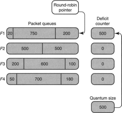
Consider the example illustrated in Figures 14.12 and 14.13. We assume that the quantum size of all flows is 500 and that there are four flows. In Figure 14.12 the round-robin pointer points to the queue of F1; the algorithm adds the quantum size to the deficit counter of F1, which is now at 500. Thus F1 has sufficient funds to send the packet at the head of its queue (of size 200) but not the second packet, of size 750. Thus the remainder (300) is left in F1’s deficit account and the algorithm skips to F2, leaving the picture shown in Figure 14.13.

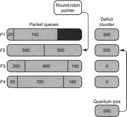
Thus in the second round, the algorithm will send the packet at the head of F2’s queue (leaving a deficit of 0), the packet at the head of F3’s queue (leaving a deficit of 400), and the packet at the head of F4’s queue (leaving a deficit of 320). It then returns to F1’s queue. F1’s deficit counter now goes up to 800; this reflects a past account balance of 300 plus a fresh deposit of 500. The algorithm then sends the packet of size 750 and the packet of size 20. Assume that no more packets arrive to F1’s queue than are shown in Figure 14.13. Thus since the F1 queue is empty, the algorithm skips to F2.

Curiously, when skipping to F2, the algorithm does not leave behind the deficit of 800 – 750 – 20 = 30 in F1’s queue. Instead, it zeroes out F1’s deficit counter. Thus the deficit counter is a somewhat curious bank account that is zeroed unless the account holder can prove a “need” in terms of a nonempty queue. Perhaps this is analogous to a welfare account.

14.6.3 Implementation and Extensions of Deficit Round-Robin

As described, DRR has one major implementation problem. The algorithm may visit a number of queues that have no packets to send. This would be very wasteful if the number of possible queues is much larger than the number of active queues. However, there is a simple way to avoid idle skipping of inactive queues by adding redundant state for speed (P12).

More precisely, the algorithm maintains an auxiliary queue, ActiveList, which is a list of indices of queues that contain at least one packet. In the example, F1, which was at the head of ActiveList, is removed from ActiveList after its last packet is serviced. If F1’s packet queue were nonempty, the algorithm would place F1 at the tail of ActiveList and keep track of any unused deficit. Notice that this prevents a flow from getting quantum added to its account while the flow is idle.

Note that DRR shares bandwidth among flows in proportion to quantum sizes. For example, suppose there are three flows, F1, F2, and F3, with respective quantum sizes 2, 2, and 3, who have reservations. Then if all three are active, F2 should get a fraction $\frac{2}{2+2+3}=2/7$ of the output-link bandwidth. If, for example, F3 is idle, then F2 is guaranteed the fraction $\frac{2}{2+2}=1/2$ of the output-link bandwidth. In all cases, a flow is guaranteed a minimum bandwidth, measured over the period the flow is active, that is proportional to the ratio of its quantum size to the sum of the quantum sizes of all other reservations.

How efficient is the algorithm? The cost to dequeue a packet is a constant number of instructions as long as each flow’s quantum is greater than a maximum-size packet. This ensures that a packet is sent every time a queue is visited. For example, if the quantum size of a flow is 1, the algorithm would have to visit a queue 100 times to send a packet of size 100. Thus if the maximum packet size is 1500 and flow F1 is to receive twice the bandwidth as flow F2, we may arrange for the quantum of F1 to be 3000 and the quantum of F2 to be 1500. Once again, in terms of our principles, we note that avoiding the generality (P7) of arbitrary quantum settings allows a more efficient implementation.

EXTENSIONS OF DEFICIT ROUND-ROBIN

We now consider two extensions of DRR: hierarchical DRR and DRR with a single priority queue.

HIERARCHICAL DEFICIT ROUND-ROBIN

An interesting model for bandwidth sharing is introduced in the so-called class-based queuing (CBQ) scheme [FJ95]. The idea is to specify a hierarchy of users that can share an output link. For example, a transatlantic link may be shared by two organizations in proportion to the amount each pays for the link. Consider two organizations, A and B, who pay, respectively, 70% and 30% of the cost of a link and so wish to have assured bandwidth shares in that ratio. However, within organization A there are two main traffic types: Web users and others. Organization A wishes to limit Web traffic to get only 40% of A’s share of the traffic when other traffic from A is present. Similarly, B wishes video traffic to take no more than 50% of the total traffic when other traffic from B is present (Figure 14.14).

Suppose at a given instant organization A’s traffic is only Web traffic and organization B has both video and other traffic. Then A’s Web traffic should get all of A’s share of the bandwidth (say, 0.7 Mbps of a 1-Mbps link); B’s video traffic should get 50% of the remaining share, which is 0.15 Mbps. If other traffic for A comes on the scene, then the share of A’s Web traffic should fall to 0.7 * 0.4 = 0.28 Mbps. Class-based queuing is easy to implement using a hierarchical DRR scheduler for each node in the CBQ tree. For example, we would use a DRR scheduler to divide traffic between A and B. When A’s queue gets visited, we run the DRR scheduler for within A, which then visits the Web queue and the other traffic queue and serves them in proportion to their quanta.

DEFICIT ROUND-ROBIN PLUS PRIORITY

A simple idea implemented by Cisco systems (and called Modified DRR, or MDRR) is to combine DRR with priority to allow minimal delay for voice over IP. The idea, depicted in Figure 14.15, allows up to eight flow queues for a router. A packet is placed in a queue based on bits in the IP TOS fields called the IP precedence bits. However, queue 1 is a special queue typically reserved for voice over IP. There are two modes: In the first mode, Queue 1 is given strict priority over the other queues. Thus in the figure, we would serve all three of queue l’s packets before alternating between queue 2 and queue 3. On the other hand, in alternating priority mode, queue 1 visits alternate with visits to a DRR scan of the remaining queues. Thus in this mode, we would first serve queue 1, then queue 2, then queue 1, then queue 3, etc.

14.7 SCHEDULERS THAT PROVIDE DELAY GUARANTEES

So far we have considered only schedulers that provide bandwidth guarantees across multiple queues. Our only exception is MDRR, which is an ad hoc solution. We now consider providing delay bounds. The situation is analogous to a number of chefs sharing an oven, as shown in Figure 14.16. The frozen-food chef (analogous to, say, FTP traffic) cares more about throughput and less about delay; the regular chef (analogous to, say, Telnet traffic) cares about delay, but for the fast-food chef (analogous to video or voice traffic) a small delay is critical for business.

In practice, most routers implement some form of throughput sharing using algorithms such as DRR. However, almost no commercial router implements schedulers that guarantee delay bounds. The result is that video currently works well sometimes, badly at other times. This may be unacceptable for commercial use. One answer to this problem is to have heavily underutilized links and to employ ad hoc schemes like MDRR. This may work if bandwidth becomes plentiful. However, traffic does go up to compensate for increased bandwidth; witness the spurt in traffic due to MP3 and Napster traffic.

In theory, the simulated bit-by-bit round-robin algorithm [DKS89] we have already mentioned guarantees isolation and delay bounds. Thus it was used as the basis for the IntServ proposal as a scheduler that could integrate video, voice, and data. However, bit-by-bit round- robin, or weighted fair queuing (WFQ), is currently very expensive to implement. Strict WFQ takes O(n) time per packet, where n is the number of concurrent flows. Recent approximations, which we will describe, take O(log(n)) time. The seminal results in reducing the overhead from O(n) to O(log n) were due to Staliadis and Verma [SV96] and Bennett and Zhang [BZ96], based on modifications to the bit-by-bit discipline. We will, however, present a version based on another scheme, called virtual clock, which we believe is simpler to understand.

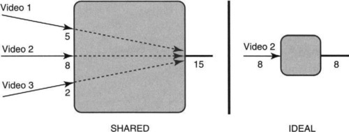
Before we study how to implement a delay bound, let us consider what an ideal delay bound should be (Figure 14.17). The left figure shows three video flows that traverse a common output link; the flows have reserved 5, 8, and 2 bandwidth units, respectively, of a 15-unit output link. The right figure shows the ideal “view” of Video 2 if it had its own dedicated router with an output link of 8 units. Thus the ideal delay bound is the delay that a flow would have received in isolation, assuming an output-link bandwidth equal to its own reservation.

Suppose the rate of flow F is r. What is the departure time of a packet p of F arriving at a router dedicated to F that always transmits at r bits per second? Well, if p arrives before the previous packet from flow F (say, prev) is transmitted, then p has to wait for prev to depart; otherwise p gets transmitted right away. Thus in an ideal system, packet p will depart by: Maximum(Arrival Time(p), Departure Time(prev)) + Length(p)/r. This recursive equation can easily be solved if we know the arrival times of all packets in flow F up to and including packet p.

Returning to Figure 14.17, if the shared system on the left must emulate the isolated system, it must service every packet before its departure time in the ideal system. In other words, as every packet arrives, we can calculate its deadline in the ideal system as in the preceding paragraph. If the shared system meets all the ideal packet deadlines, then the shared system is as good as or better than the isolated system on the right of Figure 14.17!

We may now consider using a very famous form of real-time scheduler called earliest deadline first. The classical idea is that if we wish to meet deadlines, we sort the deadlines of all the packets at the head of each flow queue and send the packet with the earliest deadline first. The corresponding packet scheduler, called virtual clock, was first introduced by Lixia Zhang [Zha91].

It was first proved [FP95] that virtual clock does a fine job of meeting deadlines. However, it does not quite emulate the system at the right of Figure 14.17 in terms of bandwidth fairness on short time scales. A flow can be locked out for a large amount of time based on past behavior. Consider the example shown in Figure 14.18. Two flows, Flow 1 and Flow 2, are assigned rates of half the link bandwidth each, where the link bandwidth is 1. Assume that Flow 1 has a large supply of packets starting from time 0, while Flow 2’s queue is empty until time 100, when it receives a large supply of packets. Thus from time 0 to time 100, since Flow 1 is the only active queue, virtual clock will send 100 packets of size 1 each from Flow 1. The first packet of Flow 1 will have ideal deadline 2, the second 4, and the 100th will have deadline 200. Thus by the time we reach time 100, Flow l’s 101st packet has ideal deadline 202.

If we now bring on 100 packets of Flow 2 at time 100, Flow 2’s packets have deadlines 102,104,106,…, and the 50th packet of Flow 2 has deadline 200. Thus during the period from 100 to 150, Flow 2 has taken all the link bandwidth, despite the presence of Flow 1 packets. This hardly looks like the model of Figure 14.17, at least from time 100 to time 150. Notice that packets are all sent within their ideal delays and that even the bandwidth given to both flows is equal across the period from 0 to 150. Unfortunately, we don’t want this behavior. We don’t want Flow 1 to be penalized, because in the past, when other flows were not present, it took more bandwidth than it needed.

There is a very simple fix for this problem, which was described concurrently in Cobb et al. [CGE96] and Suri et al. [SVC97]. Let us start by calling a flow oversubscribed if the flow sends at more than its reserved rates during short periods, as Flow 1 does in Figure 14.18. One can see that an ordinary virtual clock has a throughput unfairness problem because the deadlines of oversubscribed flows can exceed real time by an unbounded amount. For example, Flow l’s deadline can grow without bound if we increase the time when Flow 1 is the only active flow in Figure 14.18.

A careful examination shows that to guarantee delay bounds for other flows, we need only ensure that oversubscribed flow deadlines exceed real time by some threshold δ, where δ is the time taken to send a maximum-size packet at the smallest rate of any flow. For example, in Figure 14.18, this is 1/0.5, which is 2. Thus to guarantee delay bounds we only need ensure that the virtual clock of an oversubscribed flow is 2 more than real time. To make the difference go up to 100, as in Figure 14.18, is overkill.

To implement this limited “overshoot,” we can pull all oversubscribed deadlines back when time advances. Alternately, we can use a famous problem-solving technique and do a mental reversal. This allows us to see another relativistic degree of freedom (P13). Instead of pulling back a potentially large set of oversubscribed flows, we can “leap forward” the single counter representing real time. More precisely, we advance the real-time counter to be within δ of the smallest deadline whenever the smallest deadline exceeds the real-time counter by δ. Of course, now the “real-time” counter no longer represents “real-time,” but is only the reference “clock” used to stamp deadlines for future packets. The single clock adjustment is more efficient than adjusting multiple deadlines.

For example, using this new mechanism in Figure 14.18, the deadline of the 101st packet of Flow 1 at time 100 would become only 102, and not 202 as in the unmodified scheme. This ensures that Flow 1 and Flow 2 will share the link evenly in the period from time 100 to time 150.

The net result is that the leap-forward version of the virtual clock behaves just as well as ideal bit-by-bit schemes, and it takes O(log(n)) work. The logarithmic overhead is needed only for sorting deadlines using, say, a heap [CLR90]). Leaping forward is also efficient because we can access the element with the smallest tag directly from the top of the heap in constant time. What is the cost of sorting using a heap?

Recall that a d-heap is a tree in which each node of the tree contains d children and each node has a value smaller than the values contained in all its children. If the values in the leaves of the tree are deadlines, then the root contains the earliest deadline. When the earliest deadline flow is scheduled, its leaf deadline value is updated. This can change its parent value, and its parent’s parent value, and so on, up to the root. In software, a value of d greater than 2 is not much help, because each of the d children of a node must be compared when any child value changes. However, in hardware, if the d-children are stored in contiguous memory locations, then for values of d up to, say, 32, the hardware can retrieve 32 consecutive memory locations in a single wide memory access of around 1024 bits. Simple combinatorial logic within the chip can then calculate the minimum of these 32 values within the time for a memory access.

Since an update can require changing all parent values in a path from the leaf to the root, and changing each parent value takes one memory access to read and one to write, the worst-case number of memory accesses is equal to twice the maximum height of a 32-way heap, which is log₃ 2N, where N is the number of flows. Thus for N less than 32³ = 32K, the calculation of the minimum will take only six memory accesses. Thus the log N term per packet can be made very small in practice by using a large radix for the logarithm.

In terms of our principles, we are using an efficient data structure (P15) and are adding hardware (P5) in the form of a special-purpose sorting chip. The chip in turn uses wide memories and locality (P5b, exploit locality) to reduce memory access times.

A second technique to build heaps does not use wide words but uses pipelining. It is described in the exercises for Chapter 2. Note that these two solutions to making a fast heap represent two of the three memory subsystem design strategies (P5a, b, pipelining and wide word parallelism) described in Chapters 3 and 2.

In the case of both DRR and virtual clock, the basic idea works fine if all reserved rates are within small multiples of each other. However, if rates can vary by orders of magnitude (from, say, telemetry applications to video), both schemes introduce a peculiar form of burstiness described in Bennett and Zhang [BZ96]. This burstiness can be fixed using a technique of two queues first introduced in Bennett and Zhang [BZ96] and also used in Suri et al. [SVC97]. However, it adds implementation complexities of its own and may not be needed in practice.

If hardware is not available and the log n cost is significant, another possible approach [SVC97] is to trade accuracy in deadlines for reduced computation (P3b). For example, suppose your deadlines were originally 100.13,115.27,61 and we round up the deadlines (tags) to whole numbers 101,116,61. This reduces the range of numbers to be sorted, which can be exploited by bucket-sorting techniques to reduce sorting overhead. It can also be shown that the reduced deadline accuracy introduces only a small additive penalty to the delay bound.

A second approach to reduce computation, by relaxing specifications (P3b), is described in Ramabhadran and Pasquale [RP03]. While there are no worst-case delay guarantees, the scheme appears to provide good delay bounds in most cases, with computation time that is only slightly worse than for DRR.

14.8 SCALABLE FAIR QUEUING

Using multiple queues for each flow, we have seen that: (i) a constant-time algorithm (DRR) can provide bandwidth guarantees for QoS even using software and (ii) a logarithmic time- overhead algorithm can provide bandwidth and delay guarantees; further, the logarithmic overhead can be made negligible using extra hardware to implement a priority queue. Thus it would seem that QoS is easy to implement in routers ranging from small edge routers to the bigger backbone (core) routers.

Unfortunately, studies by Thompson et al. [TMW97] of backbone routers show there to be around 250,000 concurrent flows. With increasing traffic, we expect this number to grow to a million and possibly larger as Internet speed and traffic increase. Keeping state for a million flows can be a difficult task in backbone routers. If the state is kept in SRAM, the amount of memory required can be expensive; if the state is kept in DRAM, state lookup could be slow.

More cogently, advocates of Internet scaling and aggregation point out that Internet routing currently uses only around 150,000 prefixes for over 100 million nodes. Why should QoS require so much state when none of the other components of IP do? In particular, while the QoS state may be manageable today, it might represent a serious threat to the scaling of the Internet. Just as prefixes aggregate routes for multiple IP addresses, is there a way to aggregate flow state?

Aggregation implies that backbone routers will treat groups of flows in identical fashion. Aggregation requires that (i) it must be reasonable for the members of the aggregated group to be treated identically and (ii) there must be an efficient mapping from packet headers to aggregation groups. For example, in the case of IP routing, (i) a prefix aggregates a number of addresses that share the same output link, often because they are in the same relative geographic area, and (ii) longest matching prefix provides an efficient mapping from destination addresses in headers to the appropriate prefix.

There are three interesting proposals to provide aggregated QoS, which we describe briefly: random aggregation (stochastic fair queuing), aggregation at the network edge (DiffServ), and aggregation at the network edge together with efficient policing of misbehaving flows (core stateless fair queuing).

14.8.3 Edge Aggregation with Policing

Using edge aggregation, two flows (say, F1 and F2) that have reserved bandwidth (say, B₁ and B₂ respectively) could be aggregated into a class that has nominally reserved some bandwidth, which is B ≥ B₁ + B₂ for all flows in the class. Consider Figure 14.19. Suppose F1 decides to oversubscribe and to send at a rate greater than B. The edge router ER in Figure 14.19 may currently have sufficient bandwidth to allow all packets of flow F1 and F2 through. Unfortunately, when this aggregated class reaches the backbone (core) router CR, suppose the core router is limited in bandwidth and must drop packets. Ideally, CR should only drop oversubscribed flows like F1 and let all of F2’s packets through.

How, though, can CR tell which flows are oversubscribed? It could do so by keeping state for all flows passing through, but that would defeat scaling. A clever idea, called core-stateless fair queuing [SSZ], makes the observation that the edge router ER has sufficient information to distinguish the oversubscribed flows. Thus ER can, using principle P10, pass information in packet headers to CR.

How, though, should CR handle oversubscribed flows? Dropping all such marked packets may be too severe. If there is enough bandwidth for some oversubscribed flows, it seems reasonable for CR to drop in proportion to the degree a flow is oversubscribed. Thus ER should pass a value in the packet header of a flow that is proportional to the degree a flow is oversubscribed. To implement this idea, CR can drop randomly (P3a), with a drop probability that is proportional to the degree of oversubscription. While this has some error probability, it is close enough. Most importantly, random dropping can be implemented without CR keeping any state per flow. In effect, CR is implementing RED, but with the drop probability computed based on a packet header field set by an edge router.

While core-stateless is a nice idea, we note that unlike SFQ (which can be implemented in isolation without cooperation between routers) and DiffServ (which has mustered sufficient support for its standardized use of the TOS field), core-stateless fair queuing is, as of now, only a research proposal [SSZ].

14.9 SUMMARY

In this chapter, we attacked another major implementation bottleneck for a router: scheduling data packets to reduce the effects of congestion, to provide fairness, and to provide quality- of-service guarantees to certain flows. We worked our way upward from schemes, such as RED, that provide congestion feedback to schemes that provide QoS guarantees in terms of bandwidth and delay. We also studied how to scale QoS state to core routers using aggregation techniques such as DiffServ.

A real router will often have to choose various combinations of these individual schemes. Many routers today offer RED, token bucket policing, and multiple queues and DRR. However, the major point is that all these schemes, with the exception of the schemes that provide delay bounds, can be implemented efficiently; even schemes that provide delay bounds can be implemented at the cost of fairly simple added hardware. A number of combination schemes can also be implemented efficiently using the principles we have outlined. The exercises explore some of these combinations.

To make this chapter self-contained, we devoted a great deal of the discussion to explanations of topics, such as congestion control and resource reservation, that are really peripheral to the main business of this book. What we really care about is the use of our principles to attack scheduling bottlenecks. Lest that be forgotten, we remind you as always, of the summary, in Figure 14.2 of the techniques used in this chapter and the corresponding principles.

14.10 EXERCISES

1. Consider what happens if there are large variations in the reserved bandwidths of flows, for example, F1 with a rate of 1000 and F2,…, Fn with a rate of 1. Assuming that all flows have the same minimum packet size, show that flow F1 can be locked out for a long period.

2. Consider the simple idea of sending one packet for each queue with enabled quantum for each round in DRR. In other words, we interleave the packets sent in various queues during a DRR round rather than finishing a quantum’s worth for every flow. Describe how to implement this efficiently.

3. Work out the details of implementing a hierarchical DRR scheme.

4. Suppose an implementation wishes to combine DRR with token bucket shaping on the queues as well. How can the implementation ensure that it skips empty queues (a DRR scan should not visit a queue that has no token bucket credits)?

5. Describe how to efficiently combine DRR with multiple levels of priority. In other words, there are several levels of priority; within each level of priority, the algorithm runs DRR.

6. Suppose that the required bandwidths of flows vary by an order of magnitude in DRR. What fairness problems can result? Suggest a simple fix that provides better short-term fairness without requiring sorting.