
Principles in Action
System architecture and design, like any art, can only be learned by doing. … The space of possibilities unfolds only as the medium is worked.
— CARVER MEAD AND LYNN CONWAY
Having rounded up my horses, I now set myself to put them through their paces.
— ARNOLD TOYNBEE
The previous chapter outlined 15 principles for efficient network protocol implementation. Part II of the book begins a detailed look at specific network bottlenecks such as data copying and control transfer. While the principles are used in these later chapters, the focus of these later chapters is on the specific bottleneck being examined. Given that network algorithmics is as much a way of thinking as it is a set of techniques, it seems useful to round out Part I by seeing the principles in action on small, self-contained, but nontrivial network problems.
Thus this chapter provides examples of applying the principles in solving specific networking problems. The examples are drawn from real problems, and some of the solutions are used in real products. Unlike subsequent chapters, this chapter is not a collection of new material followed by a set of exercises. Instead, this chapter can be thought of as an extended set of exercises.
In Section 4.1 to Section 4.15, 15 problems are motivated and described. Each problem is followed by a hint that suggests specific principles, which is then followed by a solution sketch. There are also a few exercises after each solution. In classes and seminars on the topic of this chapter, the audience enjoyed inventing solutions by themselves (after a few hints were provided), rather than directly seeing the final solutions.
4.1 BUFFER VALIDATION OF APPLICATION DEVICE CHANNELS
Usually, application programs can only send network data through the operating system kernel, and only the kernel is allowed to talk to the network adaptor. This restriction prevents different applications from (maliciously or accidentally) writing or reading each other’s data. However, communication through the kernel adds overhead in the form of system calls (see Chapter 2). In application device channels (ADCs), the idea is to allow an application to send data to and from the network by directly writing to the memory of the network adaptor. Refer to Chapter 5 for more details. One mechanism to ensure protection, in lieu of kernel mediation, is to have the kernel set up the adaptor with a set of valid memory pages for each application. The network adaptor must then ensure that the application’s data can only be sent and received from memory in the valid set.
In Figure 4.1, for example, application P is allowed to send and receive data from a set of valid pages X, Y, …, L, A. Suppose application P queues a request to the adaptor to receive the next packet for P into a buffer in page A. Since this request is sent directly to the adaptor, the kernel cannot check that this is a valid buffer for P. Instead, the adaptor must validate this request by ensuring that A is in the set of valid pages. If the adaptor does not perform this check, application P could supply an invalid page belonging to some other application, and the adaptor would write P’s data into the wrong page. The need for a check leads to the following problem.

PROBLEM
When application P does a Receive, the adaptor must validate whether the page belongs to the valid page set for P. If the set of pages is organized as a linear list [DDP94], then validation can cost O(n), where n is the number of pages in the set. For instance, in Figure 4.1, since A is at the end of the list of valid pages, the adaptor must traverse the entire list before it finds A. If n is large, this can be expensive and can slow down the rate at which the adaptor can send and receive packets. How can the validation process be sped up? Try thinking through the solution before reading the hint and solutions that follow.
Hint: A good approach to reduce the complexity of validation is to use a better data structure than a list (P15). Which data structure would you choose? However, one can improve worst-case behavior even further and get smaller constant factors by using system thinking and by passing hints in interfaces (P9).
An algorithmic thinker will immediately consider implementing the set of valid pages as a hash table instead of a list. This provides an O(1) average search time. Hashing has two disadvantages: (1) good hash functions that have small collision probabilities are expensive computationally; (2) hashing does not provide a good worst-case bound. Binary search does provide logarithmic worst-case search times, but this is expensive (it also requires keeping the set sorted) if the set of pages is large and packet transmission rates are high. Instead, we replace the hash table lookup by an indexed array lookup, as follows (try using P9 before you read on).
SOLUTION
The adaptor stores the set of valid pages for each application in an array, as shown in Figure 4.2. This array is updated only when the kernel updates the set of valid pages for the application. When the application does a Receive into page A, it also passes to the adaptor a handle (P9). The handle is the index of the array position where A is stored. The adaptor can use this to quickly confirm whether the page in the Receive request matches the page stored in the handle. The cost of validation is a bounds check (to see if the handle is a valid index), one array lookup, and one compare.
EXERCISES
• Is the handle a hint or a tip? Let’s invoke principle P1: If this is a handle, why pass the page number (e.g., A) in the interface? Why does removing the page number speed up the confirmation task slightly?
• To find the array corresponding to application P normally requires a hash table search using P as the key. This weakens the argument for getting rid of the hash table search to check if the page is valid—unless, of course, the hash search of P can be finessed as well. How can this be done?
4.2 SCHEDULER FOR ASYNCHRONOUS TRANSFER MODE FLOW CONTROL
In asynchronous transfer mode (ATM), an ATM adaptor may have hundreds of simultaneous virtual circuits (VCs) that can send data (called cells). Each VC is often flow controlled in some way to limit the rate at which it can send. For example, in rate-based flow control, a VC may receive credits to send cells at fixed time intervals. On the other hand, in credit-based flow control [KCB94, OSV94], credits may be sent by the next node in the path when buffers free up.
Thus, in Figure 4.3 the adaptor has a table that holds the VC state. There are four VCs that have been set up (1, 3, 5, 7). Of these, only VCs 1, 5, and 7 have any cells to send. Finally, only VCs 1 and 7 have credits to send cells. Thus the next cell to be sent by the adaptor should be from either one of the eligible VCs: 1 or 7. The selection from the eligible VCs should be done fairly, for example, in round-robin fashion. If the adaptor chooses to send a cell from VC 7, the adaptor would decrement the credits of VC 7 to 1. Since there are no more cells to be sent, VC 7 now becomes ineligible. Choosing the next eligible VC leads to the following problem.
PROBLEM
A naive scheduler may cycle through the VC array looking for a VC that is eligible. If many of the VCs are ineligible, this can be quite inefficient, for the scheduler may have to step through several VCs that are ineligible to send one cell from an eligible VC. How can this inefficiency be avoided?
Hint: Consider invoking P12 to add some extra state to speed up the scheduler main loop. What state can you add to avoid stepping through ineligible VCs? How would you maintain this state efficiently?
SOLUTION
Maintain a list (Figure 4.4) of eligible VCs in addition to the VC table of Figure 4.3. The only problem is to efficiently maintain this state. This is the major difficulty in using P12. If the state is too expensive to maintain, the added state is a liability and not an asset. Recall that a VC is eligible if it has both cells to send and has credits. Thus a VC is removed from the list after service if VC becomes inactive or has no more credits; if not, the VC is added to the tail of the list to ensure fairness. A VC is added to the tail of the list either when a cell arrives to an empty VC cell queue or when the VC has no credits and receives a credit update.

EXERCISES
• How can you be sure that a VC is not added multiple times to the eligible list?
• Can this scheme be generalized to allow some VCs to get more opportunities to send than other VCs based on a weight assigned by a manager?
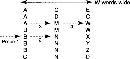
4.3 ROUTE COMPUTATION USING DIJKSTRA’S ALGORITHM
How does a router S decide how to route a packet to a given destination D? Every link in a network is labeled with a cost, and routers like S often compute the shortest (i.e., lowest-cost) paths to destinations within a local domain. Assume the cost is a small integer. Recall from Chapter 2 that the most commonly used routing protocol within a domain is OSPF based on link state routing.
In link state routing, every router in a subnet sends a link state packet (LSP) that lists its links to all of its neighbors. Each LSP is sent to every other router in the subnet. Each router sends its LSP to other routers using a primitive flooding protocol [Per92]. Once every router receives an LSP from every router, then every router has a complete map of the network. Assuming the topology remains stable, each router can now calculate its shortest path to every other node in the network using a standard shortest-path algorithm, such as Dijkstra’s algorithm [CLR90].
In Figure 4.5, source S wishes to calculate a shortest-path tree to all other nodes (A, B, C, D) in the network. The network is shown on the left frame in Figure 4.5 with links numbered with their cost. In Dijkstra’s algorithm, S begins by placing only itself in the shortest-cost tree. S also updates the cost to reach all its direct neighbors (e.g., B, A). At each iteration, Dijkstra’s algorithm adds to the current tree the node that is closest to the current tree. The costs of the neighbors of this newly added node are updated. The process repeats until all nodes in the network belong to the tree.

For instance, in Figure 4.5, after adding S, the algorithm picks B and then picks A. At this iteration, the tree is as shown on the right in Figure 4.5. The solid lines show the existing tree, and the dotted lines show the best current connections to nodes that are not already in the tree. Thus since A has a cost of 2 and there is a link of cost 3 from A to C, C is labeled with 5. Similarly, D is labeled with a cost of 2 for the path through B. At the next iteration, the algorithm picks D as the least-cost node not already in the tree. The cost to C is then updated using the route through D. Finally, C is added to the tree in the last iteration.
This textbook solution requires determining the node with the shortest cost that is not already in the tree at each iteration. The standard data structure to keep track of the minimum-value element in a dynamically changing set is a priority queue. This leads to the following problem.
PROBLEM
Dijkstra’s algorithm requires a priority queue at each of N iterations, where N is the number of network nodes. The best general-purpose priority queues, such as heaps [CLR90], take O(log N) cost to find the minimum element. This implies a total running time of O(N log N) time. For a large network, this can result in slow response to failures and other network topology changes. How can route computation be speeded up?
Hint: Consider exploiting the fact that the link costs are small integers (P14) by using an array to represent the current costs of nodes. How can you efficiently, at least in an amortized sense, find the next minimum-cost node to include in the shortest-path tree?
SOLUTION
The fact that the link costs are small integers can be exploited to construct a priority queue based on bucket sorting (P14). Assume that the largest link cost is MaxLinkCost. Thus the maximum cost of a path can be no more than Diam * MaxLinkCost, where Diam is the diameter of the network. Assume Diam is also a small integer. Thus one could imagine using an array with a location for every possible cost c in the range 1… Diam * MaxLinkCost. If during the course of Dijkstra’s algorithm the current cost of a node X is c, then node X can be placed in a list pointed to by element c of the array (Figure 4.6). This leads to the following algorithm.

Whenever a node X changes its cost from c to c′, node X is removed from the list for c and added to the list for c′. But how is the minimum element to be found? This can be done by initializing a pointer called CurrentMin to 0 (which corresponds to the cost of S). Each time the algorithm wishes to find the minimum-cost node not in the tree, CurrentMin is incremented by 1 until an array location is reached that contains a nonempty list. Any node in this list can then be added to the tree. The algorithm costs O(N + Diam * MaxLinkCost) because the work done in advancing CurrentMin can at most be the size of the array. This can be significantly better than N log N for large N and small values of Diam and MaxLinkCost.
A crucial factor in being able to efficiently use a bucket sort priority queue of the kind described earlier is that the node costs are always ahead of the value of CurrentMin. This is a monotonicity condition. If it were not true, the algorithm would start checking for the minimum from 1 at each iteration, instead of starting from the last value of CurrentMin and never backing up. The monotonicity condition is fairly obvious for Dijktra’s algorithm because the costs of nodes not already in the tree have to be larger than the costs of nodes that are already in the tree.
Figure 4.6 shows the state of the bucket sort priority queue after A has been added to the tree. This corresponds to the right frame of Figure 4.5. At this stage, CurrentMin = 2, which is the cost of A. At the next iteration, CurrentMin will advance to 3, and D will be added to the tree. This will result in the C’s cost being reduced to 4. We thus remove C from the list in position 5 and add it to the empty list in position 4. CurrentMin is then advanced to 4, and C is added to the tree.
EXERCISES
• The algorithm requires a node to be removed from a list and added to another, earlier list. How can this be done efficiently?
• In Figure 4.6, how can the algorithm know that it can terminate after adding C to the tree instead of advancing to the end of the long array?
• In networks that have failures, the concept of diameter is a highly suspect one because the diameter could change considerably after a failure. Consider a wheel topology where all N nodes have diameter 2 through a central spoke node; if the central spoke node fails, the diameter goes up to N/2. In actual practice the diameter is often small. Can this cause problems in sizing the array?
• Can you circumvent the problem of the diameter completely by replacing the linear array of Figure 4.6 with a circular array of size MaxLinkCostl Explain. The resulting solution is known as Dial’s algorithm [AMO93].
4.4 ETHERNET MONITOR USING BRIDGE HARDWARE
Alyssa P. Hacker is working for Acme Networks and knows of the Ethernet bridge invented at Acme. A bridge (see Chapter 10) is a device that can connect together Ethernets. To forward packets from one Ethernet to another, the bridge must look up the 48-bit destination address in an Ethernet packet at high speeds.
Alyssa decides to convert the bridge into an Ethernet traffic monitor that will passively listen to an Ethernet and produce statistics about traffic patterns. The marketing person tells her that she needs to monitor traffic between arbitrary source-destination pairs. Thus for every active source-destination pair, such as A, B, Alyssa must keep a variable PA,B that measures the number of packets sent from A to B since the monitor was started. When a packet is sent from A to B, the monitor (which is listening to all packets sent on the cable) will pick up a copy of the packet. If the source is A and the destination is B, the monitor should increment PA,B. The problem is to do this in 64 μsec, the minimum interpacket time on the Ethernet. The bottleneck is the lookup of the state PA,B associated with a pair of 48-bit addresses A, B.
Fortunately, the bridge hardware has a spiffy lookup hardware engine that can look up the state associated with a single 48-bit address in 1.4 psec. A call to the hardware can be expressed as Lookup(X, D), where X is the 48-bit key and D is the database to be searched. The call returns the state associated with X in 1.4 μsec for databases of less than 64,000 keys. What Alyssa must solve is the following problem.
PROBLEM
The monitor needs to update state for AB when a packet from A to B arrives. The monitor has a lookup engine that can look up only single addresses and not address pairs. How can Alyssa use the existing engine to look up address pairs? The problem is illustrated in Figure 4.7.

Hint: The problem requires using P4c to exploit the existing bridge hardware. Since 1.4 μsec is much smaller than 64 μsec, the design can afford to use more than one hardware lookup. How can a 96-bit lookup be reduced to a 48-bit lookup using three lookups?
A naive solution is to use two lookups to convert source A and destination B into smaller (<24-bit) indices IA and IB. The indices IA and IB can then be used to look up a two-dimensional array that stores the state for AB. This requires only two hardware lookups plus one more memory access, but it can require large amounts of memory. If there are 1000 possible sources and 1000 possible destinations, the array must contain a million entries. In practice, there may be only 20,000 active source-destination pairs. How could you make the required amount of memory proportional to the number of actual source-destination pairs?
SOLUTION
As before, first use one lookup each to convert source A and destination B into smaller (<24-bit) indices IA and IB Then use a third lookup to map from IAIB to AB state. The solution is illustrated in Figure 4.8. The third lookup effectively compresses the two-dimensional array of the naive solution. This solution is due to Mark Kempf and Mike Soha.
EXERCISES
• Can this problem be solved using only two bridge hardware lookups without requiring extra memory?
• The set of active source-destination pairs may change with time, because some pairs of addresses stop communicating for long periods. How can this be handled without keeping the state for every possible address pair that has communicated since the monitor was powered on?
4.5 DEMULTIPLEXING IN THE X-KERNEL
The x-kernel [HP91] provides a software infrastructure for protocol implementation in hosts. The x-kernel system provides support for a number of required protocol functions. One commonly required function is protocol demultiplexing. For example, when the Internet routing layer IP receives a packet, it must use the protocol field to determine whether the packet should be subsequently sent to TCP or UDP.
Most protocols do demultiplexing based on some identifier in the protocol header. These identifiers can vary in length in different protocols. For example, Ethernet-type fields can be 5 bytes while TCPport numbers are 2 bytes long. Thus the x-kernel allows demultiplexing based on variable-length protocol identifiers. When the system is initialized, the protocol routine can register the mapping between the identifier and the destination protocol with the x-kernel.
At run time, when a packet arrives the protocol routine can extract the protocol identifier from the packet and query the x-kernel demultiplexing routine for the destination protocol. Since packets can arrive at high speeds, the demultiplexing routine should be fast. This leads to the following problem.
PROBLEM
On average, the fastest way to do a lookup is to use a hash table. As shown in Figure 4.9, this requires computing some hash function on the identifier K to generate a hash index, using this index to access the hash table, and comparing the key L stored in the hash table entry with K. If there is a match, the demultiplexing routine can retrieve the destination protocol associated with key L. Assume that the hash function has been chosen to make collisions infrequent.
However, since the identifier length is an arbitrary number of bytes, the comparison routine that compares the two keys must, in general, do byte-by-byte comparisons. However, suppose the most common case is 4-byte identifiers, which is the machine word size. In this case, it is much more efficient to do a word comparison. Thus the goal is to exploit efficient word comparisons (P4c) to optimize the expected case (P11). How can this be done while still handling arbitrary protocols?
Hint: Notice that if the x-kernel has to demultiplex a 3-byte identifier, it has to use a byte-by-byte comparison routine; if the x-kernel has to demultiplex a 4-byte identifier and 4 bytes is the machine word size, it can use a word compare. The first degree of freedom that can be exploited is to have different comparison routines for the most common cases (e.g., word compares, long-word compares) and a default comparison routine that uses byte comparisons. Doing so trades some extra space for time (P4b). For correctness, however, it is important to know which comparison routine to use for each protocol. Consider invoking principles P9 to pass hints in interfaces and P2a to do some precomputation.
SOLUTION
Each protocol has to declare its identifier and destination protocol to the x-kernel when the system initializes. When this happens, each protocol can predeclare its identifier length, so the x-kernel can use a specialized comparison routines for each protocol. Effectively, information is being passed between the client protocol and the x-kernel (P9)at an earlier time (P2a). Assume that the x-kernel has a separate hash table for each client protocol and that the x-kernel knows the context for each client in order to use code specialized for that client.
EXERCISES
• Code up byte-by-byte and word comparisons on your machine and do a large number of both types of comparisons and compare the overall time taken for each.
• In the earlier ADC solution, the hash table lookup was finessed by passing an index (instead of the identifier length as earlier). Why might that solution be difficult in this case?
4.6 TRIES WITH NODE COMPRESSION
A trie is a data structure that is a tree of nodes, where each node is an array of M elements. Figure 4.10 shows a simple example with M = 8. Each array can hold either a key (e.g., KEY 1, KEY 2, or KEY 3 in Figure 4.11) or a pointer to another trie node (e.g., the first element in the topmost trie node of Figure 4.10, which is the root). The trie is used to search for exact matches (and longest-prefix matches) with an input string. Tries are useful in networking for such varied tasks as IP address lookup (Chapter 11), bridge lookups (Chapter 10), and demultiplexing filters (Chapter 8).


The exact trie algorithms do not concern us here. All one needs to know is how a trie is searched. Let c = log2 M be the chunk size of a trie. To search the trie, search first breaks the input string into chunks of size c. Search uses successive chunks, starting from the most significant, to index into nodes of the trie, starting with the root node. When search uses chunk j to index into position i of the current trie node, position i could contain either a pointer or a key. If position i contains a nonnull pointer to node N, the search continues at node N with chunk j + 1; otherwise, the search terminates.
To summarize, each node is an array of pointers or keys, and the search process needs to index into these arrays. However, if many trie nodes are sparse, there is considerable wasted space (P1). For example, in Figure 4.10, only 4 out of 16 locations contain useful information. In the worst case, each trie node could contain 1 pointer or key and there could be a factor of M in wasted memory. Assume M ≤ 32 in what follows. Even if M is this small, a 32-fold increase in memory can greatly increase the cost of the design.
An obvious approach is to replace each trie node by a linear list of pairs of the form (i, val), where val is the nonempty value (either pointer or key) in position i of the node. For example, the root trie node in Figure 4.10 could be replaced by the list (1, ptr); (7, KEY1), where ptr1 is the pointer to the bottom trie node. Unfortunately, this can slow down trie search by a factor of M, because the search of each trie node may now have to search through a list of M locations, instead of a single indexing operation. This leads to the following problem.
PROBLEM
How can trie nodes be compressed to remove null pointers without slowing down search by more than a small factor?
Hint: Despite compressing the nodes, array indexing needs to be efficient. If the nodes are compressed, how might information about which array elements are removed be represented? Consider leveraging off the fact that M is small by following P14 (exploit the small integer size) and P4a (exploit locality).
SOLUTION
Since M < 32, a bitmap of size 32 can easily fit into a computer word (P14 and P4a). Thus null pointers are removed after adding a bitmap with zero bits indicating the original positions of null pointers. This is shown in Figure 4.11. The trie node can now be replaced with a bitmap and a compressed trie node. A compressed trie node is an array that consists only of the nonnull values in the original node. Thus in Figure 4.11, the original root trie node (on the top) has been replaced with the compressed trie node (on the bottom). The bitmap contains a 1 in the first and seventh positions, where the root node contains nonnull values. The compressed array now contains only two elements, the first pointer and KEY 3. This still begs the question: How should a trie node be searched?
Since both uncompressed and compressed nodes are arrays and the search process starts with an index I into the uncompressed node, the search process must consult the bitmap to convert the uncompressed index I into a compressed index C into the compressed node. For example, if I is 1 in Figure 4.11, C should be 1; if I is 7, C should be 2. If I is any other value, C should be 0, indicating that there is only a null pointer.
Fortunately, the conversion from I to C can be accomplished easily by noting the following. If position I in the bitmap contains a 0, then C = 0. Otherwise, C is the number of 1’s in the first I bits of the bitmap. Thus if I = 7, then C = 2, since there are two bits set in the first seven bits of the bitmap.
This computation requires at most two memory references: one to access the bitmap (because the bitmap is small (P4a)) and one to access the compressed array. The calculation of the number of bits set in a bitmap can be done using internal registers (in software) or combinatorial logic (in hardware). Thus the effective slowdown is slightly more than a factor of 2 in software and exactly 2 in hardware.
EXERCISES
• How could you use table lookup (P14, P2a) to speed up counting the number of bits set in software? Would this necessarily require a third memory reference?
• Suppose the bitmap is large (say, M = 64 K). It would appear that counting the number of bits set in such a large bitmap is impossibly slow in hardware or software. Can you find a way to speed up counting bits in a large bitmap (principles P12 and P2a) using only one extra memory access? This will be extremely useful in Chapter 11.
4.7 PACKET FILTERING IN ROUTERS
Chapter 12 describes protocols that set up resources at routers for traffic, such as video, that needs performance guarantees. Such protocols use the concept of packet filters, sometimes called classifiers. Thus, in Figure 4.12 each receiver attached to a router may specify a packet filter describing the packets it wishes to receive. For example, in Figure 4.12 Receiver 1 may be interested in receiving NBC, which is specified by Filter 4. Each filter is some specification of the fields that describe the video packets that NBC sends. For example, NBC may be specified by packets that use the source address of the NBC transmitter in Germany and use a specified TCP destination and source port number.

Similarly, in Figure 4.12 Receiver m may be interested in receiving ABC Sports and CNN, which are described by Filters 1 and 7, respectively. Packets arrive at the router at high speeds and must be sent to all receivers that request the packet. For example, Receivers 1 and 2 may both wish to receive NBC. This leads to the following problem.
PROBLEM
Each receiving packet must be matched against all filters and sent to all receivers that match. A simple linear scan of all filters is expensive if the number of filters is large. Assume the number of filters is over a thousand. How can this expensive process be sped up?
Hint: One might think of optimizing the expected case by caching (P11a). However, why is caching difficult in this case? Consider adding a field (P10) to the packet header to make caching easier. Ideally, which protocol layer should this be added to? Adding a fixed well-known field for each possible video type is not a panacea because it requires global standardization, and filters can be based on other fields, such as the source address. Assume the field you add does not require globally standardized identifiers. What properties of this field must the source ensure?
SOLUTION
Caching (P11a), the old workhorse of system designers, is not very straightforward in this problem. In general, a cache stores a mapping between an input a and some output f (a). The cache then consists of a set of pairs of the form (a,f (a)). This set of pairs is stored as a database keyed by values of a. The database can be implemented as a hash table (in software) or a content-addressable memory (in hardware). Given input a and the need to calculate f(a), the database is first checked to see if a is already in the database. If so, the fast path exits with the existing value of f(a). If not, f(a) is computed using some other (possibly expensive) computation and the pair (a,f(a)) is then inserted into the cache database. Subsequent inputs with value a can then be calculated very fast.
In the packet filtering problem, the goal is to calculate the set of receivers associated with a packet P. The problem is that the output is a function of a (potentially) large number of packet header fields of P. Thus to use caching, one has to store a large portion of the headers of P associated with the set of receivers for P. Storing a mapping between 64 bytes of packet header and an output set of receivers is an expensive proposition. It is expensive in time, since searching the cache can take longer because the keys are wide. It is also clearly expensive in storage. The large storage needs in turn imply that fewer mappings can be cached for a given cache size, which leads to a poorer cache hit rate.
The ideal is to cache a mapping between one or two packet fields and the output receiver set. This would speed up cache search time and improve the cache hit rate. These fields should also preferably be in the routing header, which routers examine anyway. The problem is that there may be no such field that uniquely fingerprints packet P.
However, suppose we are system designers designing the routing protocol. We can add a field to the routing header. The problem might seem trivial if we could assign each possible stream of packets a unique global identifier. For example, if we could assign NBC identifier 1, ABC identifier 2, and CNN identifier 3, then we could cache using the identifier as the key. Such a solution would require some form of global standards committee responsible for naming every application stream. Even if that could be done, the receiver filter might ask for all NBC packets from a given source, and the filter could depend on other packet fields. This leads to the following final idea.
Change the routing header to add a flow identifier F (Figure 4.13), whose meaning depends on the source. In other words, different sources can use the same flow identifier because it is the combination of the source and the flow identifier that is unique. Thus there is no need for global standardization (or other global coordination) of flow identifiers. A flow identifier is only a local counter maintained by the source. The idea is that a sending application at the sender can ask the routing layer for a flow identifier. This identifier is added to the routing header of all the packets for this application.

As usual, when the application packet first arrives, the router does a (slow) linear search to determine the set of receivers associated with the packet header. Because identifiers are not unique across sources, the router caches the mapping using the concatenation of the packet source address and the flow identifier as the key. Clearly, correctness depends on the sender application’s not changing fields that could affect a filter without also changing the flow identifier in the packet.
EXERCISES
• What can go wrong if the source crashes and comes up again without remembering which identifiers it has assigned to different applications? What can go wrong when a receiver adds a new filter? How can these problems be solved?
• In the current solution, the flow identifier is used as a tip (Chapter 3) and not as a hint. What additional costs would be incurred if the flow identifier-source address pair is treated as a hint and not as a tip?
4.8 AVOIDING FRAGMENTATION OF LINK STATE PACKETS
The following problem actually arose during the design of the OSI and OSPF [Per92] link state routing protocols. This problem is about protocol design, as opposed to protocol implementation once the design is fixed. Despite this, it illustrates how design choices can greatly affect implementation performance.
Chapter 2 and Section 4.3 described link state routing. Recall that in link state routing, a router must send a link state packet (LSP) listing all its neighbors. The link state protocol consists of two separate processes. The first is the update process that sends link state packets reliably from router to router using a flooding protocol that relies on a unique sequence number per link state packet. The sequence number is used to reject duplicate copies of an LSP. Whenever a router receives a new LSP numbered x from source S, the router will remember number x and will reject any subsequent LSPs received from S with sequence number x. After the update process does its work, the decision process at every router applies Dijkstra’s algorithm to the network map formed by the link state packets.
While a router may have a small number of router neighbors, a router may have a large number of host computers (endnodes) that are connected directly to the router on the same LAN. For example, in Figure 4.14, router R1 has 500 endnode neighbors E1 … E500. Large LANs may even have a larger number of endnodes. This leads to the following problem.
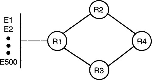
PROBLEM
At 8 bytes per endnode (6 bytes to identify the endnode and 2 bytes of cost information), the LSP can be very large (40,000 bytes for 5000 endnodes). This is much too huge for the link state packet to fit into a maximum-size frame on many commonly used data links. For example, Ethernet has a maximum size of 1500 bytes and FDDI specifies a maximum of 4500 bytes. This implies that the large LSP must be fragmented into many data link frames on each hop and reassembled at each router before it can be sent onward. This requires an expensive reassembly process at each hop to determine whether all the pieces of a LSP have been received.
It also increases the latency of link state propagation. Suppose that each LSP can fit in M data link frames, that the diameter of the network is D, and that the time to send a data link frame over a link is 1 time unit. Then with hop-by-hop reassembly, the propagation time of an LSP can be D · M. If a router did not have to wait to reassemble each LSP at each hop, the propagation delay would be only M + D. When the link state protocol was being designed, these problems were discovered by implementors reviewing the initial specification.
On the other hand, it seems impossible to propagate the fragments independently because the LSP carries a single sequence number that is crucial to the update process. Simply copying the sequence number into each fragment will not help, because that will cause the later fragments to be rejected, since they have the same sequence number as the first fragment. The problem is to make the impossible possible by shifting computation around in space to avoid the need for hop-by-hop fragmentation. Changes to the LSP routing protocol are allowed.
Hint: Does the information about all 5000 endnodes have to be in the same LSP? Consider invoking P3c to shift computation in space.
SOLUTION
If the individual fragments of the original LSP of R1 are to be propagated independently without hop-by-hop reassembly, then each fragment must be a separate LSP by itself, with a separate sequence number. This crucial observation leads to the following elegant idea.
Modify the link state routing protocol to allow any router R1 to be multiple pseudo-routers R1a, R1b, R1c (see Figure 4.15). The original set of endnodes are divided among these pseudorouters, so the LSP of each pseudo-router can fit into most data link frames without the need for fragmentation. For example, if most data link sizes are at least 576 bytes, roughly 72 endnodes can fit within a data link frame.
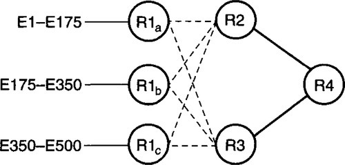
How is this concept of a pseudo-router actually realized? In the original LSP propagation, each router had a 6-byte ID that is placed in all LSPs sent by the router. To allow for pseudorouters, we change the protocol to have LSPs carry a 7-byte ID (6-byte router ID + 1-byte pseudo-router ID). The pseudo-router ID can be assigned by the actual router that houses all the pseudo-routers. By allowing 256 pseudo-routers per router, roughly 18,000 endnodes can be supported per router.
While the LSP propagation treats pseudo-routers separately, it is crucial that route computation treat the separate pseudo-routers as one router. After all, the endnodes are all directly connected to R1 in our example. But this is easily done, because all the LSPs with the same first 6 bytes can be recognized as being from the same router.
In summary, the main idea is to shift computation in space (P3c) by having the source fragment the original LSP into independent LSPs instead of having each data link do the fragmentation. This is a good example of systems thinking. Needless to say, the implementors liked this solution (invented by Radia Perlman) much better than the original approach.
EXERCISES
• How can a router assign endnodes to pseudo-routers? What happens if a router initially has a lot of endnodes (and hence a lot of pseudo-routers) and then most of the endnodes die? This can leave a lot of pseudo-routers, each of which has only a few endnodes. Why is this bad, and how can it be fixed?
• As in the relaxed-consistency examples described in Chapter 3, this solution can lead to some unexpected (but not very serious) temporary inconsistencies. Assuming a solution to the previous exercise, describe a scenario in which a given router, say, R2, can find (at some instant) that its LSP database shows the same endnode (say, E1) belonging to two pseudo-routers, R1a and R1c. Why is this no worse than ordinary LSP routing?
4.9 POLICING TRAFFIC PATTERNS
Some network protocols require that sources never send data faster than a certain rate. Instead of merely specifying the average rate over long periods of time, the protocol may also specify the maximum amount of traffic, B, in bits a source can send in any period of T seconds. This does limit the source to an average rate of B/T bits per second. However, it also limits the “burstiness” of the users’ traffic to at most one burst of size B every T units of time. For example, choosing a small value of the parameter T limits the traffic burstiness considerably. Burstiness causes problems for networks because periods of high traffic and packet loss are followed by idle periods.
If every source meets its contract (i.e., sends no more than the specified amount in the specified period), the network can often guarantee performance and ensure that no traffic is dropped and that all traffic is delivered in timely fashion. Unfortunately, this is like saying that if everyone follows the rules of the road, traffic will flow smoothly. Most people do follow the rules: some because they feel it is the right thing to do, and many because they are aware of penalties that they have to pay when caught by traffic police. Thus policing is an important part of an ordered society.
For the same reason, many designers advocate that the network should periodically police traffic to look for offenders that do not meet their contracts. Without policing, the offenders can get an unfair share of network bandwidth.
Assume that a traffic flow is identified by the source and destination address and the traffic type. Thus each router needs to ensure that a particular traffic flow sends no more than B bits in any period of T seconds. The simplest solution is for the router to use a single timer that ticks every T seconds and to count the number of bits sent in each period using a counter per flow. At the end of each period, if the counter exceeds B, the router has detected a violation.
Unfortunately, the single timer can police only some periods. For example, assume without loss of generality that the timer starts at time 0. Then the only periods checked are the periods [0, T], [T, 2T], [2T, 3T],…. This does not ensure that the source flow does not violate its contract in a period like [T/2,3T/2], which overlaps the periods that are policed. For example, in the left side of Figure 4.16, the flow sends a burst of size B just before the timer ticks at time T and sends a second burst of size B just after the timer ticks at time T.

One attempt to fix this problem is for the router to use multiple timers and counters. For example, as shown on the right of Figure 4.16, the router could use one timer that starts at 0 and a second timer that starts at time T/2. Unfortunately, the flow can still violate its contract by sending no more than B in each policed period but sending more than B in some overlapping period.
For instance, in the right frame of Figure 4.16 an offending flow sends a first burst of B at the end of the first period and a second burst of B at the start of the third period, sending 2B within a period slightly greater than T/2. Unfortunately, neither of the timers will detect the flow as being a violator. This leads to the following problem.
PROBLEM
Multiple timers are expensive and do not guarantee that the flow will not violate its traffic contract. It is easy to see that with even a single timer, the flow can send no more than 2B in any period of T seconds. One approach is simply to assume that a factor-of-2 violation is not worth the effort to police. However, suppose that bandwidth is precious on a transcontinental link and that a factor-of-2 violation is serious. How could a violating flow still be caught using only a single timer?
Hint: Consider exploiting a degree of freedom (P13) that has been assumed to be fixed in the naive solution. Do the policing intervals have to start at fixed intervals? Also consider using P3a.
SOLUTION
As suggested in the hints, the policing intervals need not be fixed. Thus, there can be an arbitrary gap between policing intervals. How should the gap be picked? Since a violating flow can pick its violating period of T to start at any instant, a simple idea is to invoke P3a to yield the following idea (Figure 4.17).

The router uses a single timer of T units and a single counter, as before. A policing interval ends with a timer tick; if the counter is greater than B, a violation is detected. Then a flag is set indicating that the timer is now used only for inserting a random gap. Then the timer is restarted for a random time interval between 0 and T. When the timer ticks, the flag is cleared and the counter is initialized, and the timer is reset for a period of T to start policing again.
EXERCISES
• Suppose the counter is initialized and maintained during the gap period as well as during policing periods. Can the router make any valid inference during such a period, even if the gap period is less than T units?
• (Open Problem): Suppose the flow is adversarial. What is a good strategy for the flow to consistently violate the contract by as high a margin as possible and still elude the randomized detector described earlier? The flow strategy can be randomized as well. A good answer should be supported by a probabilistic analysis.
4.10 IDENTIFYING A RESOURCE HOG
Suppose a device wishes to keep track of resources, like the packet memory allocated to various sources in a router. The device wants a cheap way to find the source consuming the most memory so that the device can grab memory back from such a resource hog. Figure 4.18 shows five sources with their present resource consumption of 1, 9, 30, 24, and 7 units, respectively. The resource hog is S3.
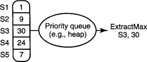
A simple solution to identify the resource hog is to use a heap. However, if the number of sources is a thousand or more, this may be too expensive at high speeds. Assume that the numbers that describe resource usage are integers in the range from 1 to 8000. Thus bucket sort techniques won’t work well because we may have to search 8000 entries to find the resource hog.
Suppose, instead, that the device does not care about the exact maximum as long as the result comes within a factor of 2 (perfect fairness is unimportant as in P3b). For example, in the figure, assume it is fine to get an answer of 24 instead of 30. This leads to the following problem.
PROBLEM
A software or hardware module needs to keep track of resources required by various users. The module needs a cheap way to find the user consuming the most resources. Since ordinary heaps are too slow, the device designers are willing to relax the system requirements (P3b) to be off by a factor of 2. Can this relaxation in accuracy requirements be translated into a more efficient algorithm?
Hint: Consider using three principles: trading accuracy for computation (P3b), using bucket sorting (P14), and using table lookups (P4b, P2a).
SOLUTION
Since the answer can be off by a factor of 2, it makes sense to aggregate users whose resources are within a factor of 2 into the same “resource usage group.” This can be a win if the resulting number of groups is much smaller than the original number of users; finding the largest group then will be faster than finding the largest user. This is roughly the same idea behind aggregation in hierarchical routing, where a number of destinations are aggregated behind a common prefix; this can make routing less accurate but reduces the number of routing entries. This leads to the following idea (try to work out the details before you read further).
Binomial bucketing can be used, as shown in Figure 4.19, where all users are grouped into buckets according to resource consumption, where bucket i contains all users whose resource consumption lies between 2i and 2i+1 – 1. In Figure 4.19, for instance, users S3 and S4 are both in the range [16,31] and hence are in the same bucket.
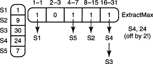
Each bucket contains an unsorted list of the resource records of all the users that fall within that bucket range. Thus in Figure 4.19, S3 and S4 are in the same list. The data structure also contains a bitmap, with one bit for every bucket, that is set if the corresponding bucket list is nonempty (Figure 4.19). Thus in Figure 4.19, the bits corresponding to buckets [1,1], [4,7], [8,15], and [16,31] are set, while the bit corresponding to [2,3] is clear.
Thus to find the resource hog, the algorithm simply looks for the bit position i corresponding to the rightmost bit set in the bitmap. The algorithm then returns the user at the head of the bucket list corresponding to position i. Thus in Figure 4.19, the algorithm would return S4 instead of the more accurate S3.
EXERCISES
• How is this data structure maintained? What happens if the resources in a user (e.g., S3) are reduced from 30 to 16? What kind of lists are needed for efficient maintenance?
• How large is each bitmap? How can finding the rightmost bit set be done efficiently?
4.11 GETTING RID OF THE TCP OPEN CONNECTION LIST
A transport protocol such as TCP [Ste94] in computer X keeps state for every concurrent conversation that X has with other computers. Recall from Chapter 2 that the technical name for the shared state between the two endpoints of a conversation is a connection. Thus if a user wishes to send mail from X to another workstation, Y, the mail program in X must first establish a connection (shared state) to the mail program in Y. A busy server like a Web server may have lots of concurrent connections.
The state in a connection consists of things like the numbers of packets sent by X that have not been acknowledged by Y. Any packets that have not been acknowledged for a long time must be retransmitted by X. To do retransmission, transport protocols typically have a periodic timer that triggers the retransmission of any packets whose acknowledgments have been outstanding for a while.
The freely available Berkeley (BSD) TCP code [Ste94] keeps a list of open connections (Figure 4.20) to examine on timer ticks in order to perform any needed retransmissions. However, when a packet arrives at X, TCP at X must also quickly determine which connection the packet belongs to in order to update the state for the connection. Each connection is identified by a connection identifier that is carried in every packet.
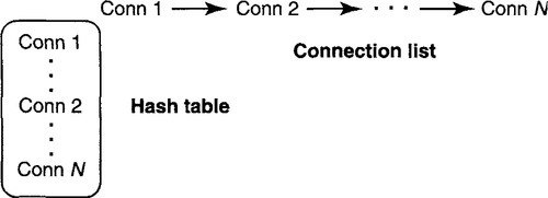
Relying on the list to determine the connection for a packet would require searching the entire list, in the worst case; this could be slow for servers with large numbers of connections. Thus the x-kernel implementation [HP91] added a hash table to the BSD implementation (P15) to efficiently map from connection identifiers in packets to the corresponding state for the connection. The hash table is an array of pointers indexed by hash value that points to lists of connections that hash to the same value. In addition, the original linked list of connections was retained for timer processing, while the hash table was supposed to speed up packet processing.
Oddly enough, measurements of the new implementation actually showed a slowdown! Careful measurements traced the problem to the fact that information about connections was stored redundantly, and this reduced the efficiency of the data cache when implemented on modern processors (see Chapter 2 for a model of a modern processor). This illustrates question Q3 in Chapter 3, where an obvious improvement to one part of the system can affect other parts of the system. Note that while main memory may be cheap, fast memory such as the data cache is often limited. Commonly used structures such as the connection list should float into the data cache as long as they are small enough to fit.
The obvious solution is to avoid redundancy. The hash table is needed for fast lookups. The timer routine must also periodically and efficiently scan through all connections. This leads to the following problem.
PROBLEM
Can you get rid of the waste caused by the explicit connection list while retaining the hash table? It is reasonable to add a small amount of extra information to the hash table. When doing so, observe that the original connection list was made doubly linked to allow easy deletion when connections terminate. But this adds storage and dilutes the data cache. How can a singly linked list be used without slowing down deletion?
Hint: The first part is easy to fix by linking the valid hash table entries in a list. The second part (avoiding the doubly linked list, which would require two pointers per hash table entry) is a bit harder.
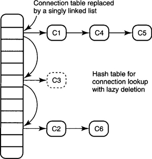
A connection list consists of nodes, each of which contains a connection ID (96 bits for IP) plus two pointers (say, 32 bits each) for easy deletion. Since the hash table is needed for fast demultiplexing, the connection list can be removed if the valid hash table entries are linked together as shown in Figure 4.21 and a pointer is kept to the head of the list. On a timer tick, the retransmit routine will periodically scan this list. Scanning the complete hash table is less efficient because the hash table may have many empty locations.
The naive solution would add two pointers to each valid hash table entry to implement a doubly linked list. Since these pointers can be hash table indexes instead of arbitrary pointers to memory, the indexes need not be larger than the size of the hash table: Even the largest hash table storing connections should require no more than 16 bits, often much less. The naive solution does well, adding at most 32 bits per entry instead of 160 bits per entry, a savings of 128 bits. However, it is possible to do better and to add only 16 bits per entry. Consider using lazy evaluation (P2b) and relaxing the specification (P3).
SOLUTION
A doubly linked list is useful only for efficient deletions. When a connection (say, Connection C3 in Figure 4.21) is terminated, the delete routine would ideally like to find the previous valid entry (i.e., the list containing Connection C1 in Figure 4.20) in order to link the previous list to the next list (i.e., the list containing C2). This would require each hash table entry to store a pointer to the previous valid entry in the list.
Instead, consider principle P3, which asks whether the system requirements can be relaxed. Normally, one assumes that when a connection terminates, its storage must be reclaimed immediately. To reclaim storage, the hash table entry should be placed in a free list, where it can be used by another connection. However, if the hash table is a little larger than strictly necessary, it is not essential that the storage used by a terminated connection be reused immediately.
Given this relaxation of requirements, the implementation can lazily delete the connection state. When a connection is terminated, the entry must be marked as unused. This requires an extra bit of state, as in P12, but is cheap. The actual deletion of unused hash table entry E involves linking the entry before E to the entry after E and also requires returning E to a free list. However, this deletion can be done on the next list traversal when the traversal encounters an unused entry.
EXERCISES
• Write pseudocode for the addition of a new connection, the termination of a connection, and the timer-based traversal.
• How can we get away with singly linked lists for the lists of connections in each hash table list?
• Hugh Hopeful is always interested in clever tricks that he never thinks through completely. He suggests a way to avoid back pointers in any doubly linked list. Suppose a node X needs to be deleted. Normally, the deletion routine is passed a handle to retrieve X, which is typically a pointer to node X. Instead, Hugh suggests that the handle be a pointer to the node before X in the linked list (except when X is the head of the list when the handle is a null pointer). Hugh claims that this allows his implementation to efficiently locate both the node prior to X and the node after X using only forward pointers. Present a counterexample to stop Hugh before he writes some buggy code.
4.12 ACKNOWLEDGMENT WITH HOLDING
Transport protocols such as TCP ensure that data is delivered to the destination by requiring that the destination send an acknowledgment (ack) for every piece of received data. This is analogous to certified mail. Packets and acks are numbered. Acks are often cumulative; an ack for a packet numbered N implicitly acknowledges all packets with numbers less than or equal to N.
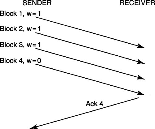
Cumulative acks allow the receiver the flexibility of not sending an ack for every received packet. Instead, acks can be batched (P2c). For example, in Figure 4.22 a file transfer program is sending file blocks, one in every packet. Blocks 1 and 2 are individually acknowledged, but blocks 3 and 4 are acknowledged with a single ack for block 4.

Reducing acks is a good thing for the sender and receiver. Although acks are small, they contain headers that must be processed by every router and the source and the destination. Further, each received packet, however small, can cause an interrupt at the destination computer, and interrupts are expensive. Thus ideally, a receiver should batch as many acks as possible. But what should the receiver batching policy be? This leads to the following problem.
PROBLEM
Ack withholding is difficult at a receiver that is not clairvoyant. In Figure 4.22, for example, if block 3 arrives first and is processed quickly, how long should the receiver wait for block 4 before sending the ack for block 3? If block 4 never arrives (because the sender has no more data to send), then withholding the ack for block 3 would cause incorrect behavior. The classical solution is to set an ack-withholding timer; when the timer expires, a cumulative ack is sent. This limits the time that an ack can be withheld.
However, the withholding timer also causes problems. Some applications are sensitive to latency. Adding an ack-withholding timer can increase latency in cases where the sender has no more data to send. If the transport protocol could be modified, what information could be added to avoid unnecessary latency and yet allow acks to be effectively batched?
Hint: In an application such as FTP, which software module “knows” that there is more data to be sent? For ack withholding, which software module would ideally like to know that there is more data to be sent? Now consider using P9 and P10.
SOLUTION
In an application such as file transfer, the sender application knows that there is more data to be sent (e.g., there will be a block 4 after block 3). The sending application may also be willing to tolerate the latency due to batching of acks. However, it is the transport module at the receiver that needs to know this information. This observation leads to a simple proposal.
The sender application passes a bit to the sender transport (in the application-transport interface) that is set when the application has more data to send. Assume that the transport protocol can be modified to carry a withhold bit. The sending transport can use the information passed by the application to set a withhold bit w in every packet that it sends; w is cleared when the sender wants an immediate ack. The moral, of course, is that it is better for the sender to telegraph his intentions than for the receiver to make guesses about the future!
For example, in Figure 4.23 the sender transport is informed by the sending file transfer application that there are four blocks to be sent. Thus the sender transport sets the withhold bit on the first three packets and clears the bit in the fourth packet. The receiver acts on this information to send one ack instead of four. On the other hand, an application that is latency sensitive can choose not to pass any information about data to be sent. Note also that the withhold bit is a hint; the receiver can choose to ignore this information and send an ack anyway. Despite its apparent cleverness, this solution is a bad idea in today’s TCP. See the exercises for details.
EXERCISES
• Another technique for reducing acks is to piggyback acks on data flowing from the receiver to the sender. To support this, most transport protocols, such as TCP, have extra fields in data packets to convey reverse ack information. However, piggybacking has the same classical trade-off between latency and piggybacking efficiency. How long should the receiver transport wait for reverse data? On the other hand, there are common applications where the sender application knows this information. How could the solution outlined earlier be extended to support piggybacking as well as ack batching?
• Recall that Chapter 3 outlined a set of cautionary questions for evaluating purported improvements. For example, Q3 asks whether a change can affect the rest of the system. Why might aggressive ack withholding interact with other aspects of the transport protocol, such as flow and congestion control [Ste94]?
4.13 INCREMENTALLY READING A LARGE DATABASE
Suppose a user continuously reads a large database stored on a Web site. The Web page can change and the reader only wants the incremental (P12a) updates since the last read of the database. Thus, in Figure 4.24 there is a database of highly popular food items that is being read constantly by readers around the world who wish to keep up with culinary fashion. Fortunately, food fashions change slowly.
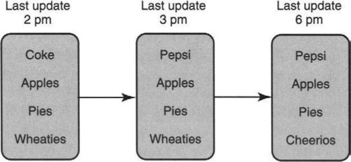
Thus a reader that last read at 2 pm and reads again at 6 pm only wants the differences: Coke to Pepsi, and Wheaties to Cheerios. If, on the other hand, a different user reads at 3 pm and then at 6 pm, she, too, only wants the difference: Wheaties to Cheerios. This leads to the following problem.
PROBLEM
Find a way for the database to efficiently perform such incremental queries. One solution is to have the database remember what each user has previously read. However, it is unreasonable for the database to remember what each user has previously read, since there may be millions of users. Find another solution that is less burdensome for the database program.
Hint: If the database does not store any information about the last Read performed by a user, then it follows that user Read requests must pass some information (P10) about the last Read request made by the same user. Passing the entire details of the last Read would be overkill and inefficient. What simple piece of information can succinctly characterize the user’s last request? Now consider adding redundant state (P12) at the database that can easily be indexed using the information passed by the user to facilitate efficient incremental query processing.
SOLUTION
As said earlier, user Read requests must pass some information (P10) about the last Read request made by the same user. The most succinct and relevant piece of information about the last user request is the time at which it was made. If user requests pass the time of the last Read, then the database needs to be organized to efficiently compute all updates after any given time. This can be done by storing copies of the database at all possible earlier times. This is clearly inefficient and can be avoided by storing only the incremental changes (P12a). This leads to the following algorithm.
Add an update history list to the database, with most recent updates closer to the head of the list. Read requests carry the time T of the last Read, so a Read request can be processed by scanning the update list from the head to find all updates after T.
For example, in Figure 4.25 the head of the update history list has the latest change (compare with Figure 4.24) at 6 pm from Wheaties to Cheerios and the next earliest change at 3 pm from Coke to Pepsi. Consider a Read request that has a last Read time of 5 pm. In this case, when scanning the list from the head, the request processing will find the 6 pm update and stop when it reaches the 3 pm update because 3 < 5. Thus the Read request will return only the first update.

EXERCISES
• If a single entry changes multiple times, a single entry change can be stored redundantly in the list, which costs space and time. What principle can you use to avoid this redundancy? Assume the database is just a collection of records and that you want each record to appear at most once in the incremental list.
• If the number of records is large or the foregoing trick is not adopted, the incremental list size will grow very big. Suggest a sensible policy for periodically reducing the size of the incremental list.
4.14 BINARY SEARCH OF LONG IDENTIFIERS
The next-generation Internet (IPv6) plans to use larger, 128-bit addresses to accommodate more Internet endpoints. Suppose the goal is to look up 128-bit addresses. Assume the algorithm works on a machine whose natural word size is 32 bits. Then each comparison of two 128-bit numbers will take 128/32 = 4 operations to compare each word individually. In general, suppose each identifier in the table is W words long. In our example, W = 4. Naive binary search will take W · log N comparisons, which is expensive. Yet this seems obviously wasteful. If all the identifiers have the same first W – 1 words, then clearly log N comparisons are sufficient. The problem is to modify binary search to take log N + W comparisons. The strategy is to work in columns, starting with the most significant word and doing binary search in that column until equality is obtained in that column. At that point, the algorithm moves to the next word to the right and continues the binary search where it left off.
Thus in Figure 4.26, which has W = 3, consider a search for the three-word identifier BMW. Pretend each character is a word. Start by comparing in the leftmost column in the middle element, as shown by the arrow labeled 1.1 Since the B in the search string matches the B at the arrow labeled 1, the search moves to the right (not shown) to compare the M in BMW with the N in the middle location of the second column. Since N < M, the search performs the second probe at the quarter position of the second column. This time the two M’s match and the search moves rightward and finds W, but (oops!) the search has found AMW, not BMW as desired. This leads to the following problem.
PROBLEM
Find some state that can be added to each element in each column that can fix this algorithm to work correctly in log N + W comparisons.
Hint: The problem is caused by the fact that when the search moved to the quarter position in column 2, it assumed that all elements in the quarter of the second column begin with B. This assumption is false in general. What state can be added to avoid making this false assumption, and how can the search be modified to use this state?
SOLUTION
The trick is to add state to each element in each column, which can constrain the binary search to stay within a guard range. This is shown in Figure 4.27. In the figure, for each word like B in the leftmost (most significant) column, add a pointer to the range of all other words that also contain B in this position. Thus the first probe of the binary search for BMW starts with the B in BNX. On equality, the search moves to the second column, as before. However, search also keeps track of the guard range corresponding to the B’s in the first column. The figure shows that the guard range includes only rows 4 through 7. This guard range is stored with the first B compared (see arrows in Figure 4.27).

Thus when the search moves to column 2 and finds that M in BMW is less than the N in BNX, it attempts to halve the range as before and to try a second probe at the third entry (the M in AMT). However, the third entry is lower than the high point of the current guard range (4 through 6, assuming the first element is numbered 1). So without doing a compare, the search tries to halve the binary search range again. This time the search tries entry 4, which is in the guard range. The search finds equality, moves to the right, and finds BMW, as desired.
In general, every multiword entry W1, W2,…, Wn will store a precomputed guard range. The range for Wi points to the range of entries that have W1, W2,…, Wi in the first i words. This ensures that on a match with Wi in the ith column, the binary search in column i + 1 will search only in this guard range. For example, the N entry in BNY (second column) has a guard range of 5–7, because these entries all have BN in the first two words.
The resulting search strategy takes log2 N + W probes if there are N identifiers. The cost is the addition of two 16-bit pointers to each word. Since most word sizes are at least 32 bits, this results in adding 32 bits of pointer space for each word, which can at most double memory usage. Besides adding state, a second dominant idea is to use precomputation (P2a) to trade a slower insertion time for a faster search. The idea is due to Butler Lampson.
EXERCISE
• (This is harder than the usual exercises.) The naive method of updating the binary search data structure requires rebuilding the entire structure (especially because of the precomputed ranges) when a new entry is added or deleted. However, the whole scheme can be elegantly represented by a binary search tree, with each node having the usual > and < pointers but also an = pointer, which corresponds to moving to the next column to the right, as shown earlier. The subtree corresponding to the = pointer naturally represents the guard range. The structure now looks like a trie of binary search trees. Use this observation and standard update techniques for balanced binary trees and tries to obtain logarithmic update times.
4.15 VIDEO CONFERENCING VIA ASYNCHRONOUS TRANSFER MODE
In asynchronous transfer mode (ATM), the network first sets up a virtual circuit through a series of switches before data can be sent. Standard ATM allows one-to-many virtual circuits, where a virtual circuit (VC) can connect a single source to multiple receivers. Any data sent by the source is replicated and sent to every receiver in the one-to-many virtual circuit.
Although it is not standardized, it is also easy to have many-to-many VCs, where every endpoint can be both a source and a receiver. The idea is that when any source sends data, the switches replicate the data to every receiver. Of course, the main problem in many-to-many VCs is that if two sources talk at the same time, then the data from the two sources can be arbitrarily interleaved at the receivers and cause confusion. This is possibly why many-to-many VCs are not supported by standards, though it is often easy for switch hardware to support many-to-many VCs.
Figure 4.28 shows a simple topology consisting of an ATM switch that connects N workstations. To showcase the bandwidth of the switch, the system designers have designed a videoconferencing application. The conferencing application can allow users at any of the N workstations to have a videoconference with each other. The application should bring up a screen (on every workstation in the conference) that displays at least the current speaker and also plays the speech of the current speaker. In addition, in the event of a conversation, it is desirable to see the expressions of the participants. The designers soon run into the following problem.

PROBLEM
The naivest solution would use up to N2 point-to-point connections between every pair of participating workstations. A better solution is shown in Figure 4.28. It uses up to N many-to-many VCs between each participating workstation and the other workstations. The video and speech of each workstation is connected by a one-to-many virtual circuit to every other participating workstation. Thus every participating workstation gets the video output of all participants and the application can choose which one (or ones) to display. Unfortunately, the ATM switch requires that bandwidth on the switch be statically divided among the N one-to-many VCs. Given a minimum bandwidth for video quality of Bmin and a total switch bandwidth of B, this limits the number of participating workstations to be less than B/Bmin. Is there a more scalable solution?
Hint: Consider exploiting the switch hardware’s ability to support many-to-many VCs (P4c). However, to prevent confusion, only one source should transmit at a time in any many-to-many VC. Instead of developing a complex protocol to ensure such a constraint, what hardware can be added (P5) to ensure this constraint?
SOLUTION
As suggested in the hint, the designers chose to exploit the many-to-many VC capability of the switch to replace N one-to-many VCs with a constant number of many-to-many VCs. This allowed the fixed switch bandwidth to scale to a large number of participants. However, this generic idea requires elaboration. How many many-to-many VCs should be used? How is the potential confusion caused by many-to-many VCs resolved? Here are the details of a solution worked out by Jon Turner at Washington University.
First, consider the use of a single many-to-many VC named C. A naive solution to the confusion problem entails a protocol (say, a round-robin protocol) that ensures that only one workstation at a time connects its video output to C. Such protocols require coordination, and the coordination adds latency and expense. Instead, as systems thinkers, the designers observed that, at a minimum, only the current speaker needs to be displayed.
Thus the designers added extra hardware (P5) in the form of a speech detector to the input at each workstation. If the detector detects significant speech activity at a workstation X, then the detector connects the video input of X to C; otherwise, the video input of X is not connected to C Since this hardware was quite cheap, the extra scalability came at a reasonable price.
Next, the designers observed that keeping a video image of the last speaker provides visual continuity in the expected case when there is a dialog between two participants. Thus instead of one many-to-many VC, they used two many-to-many VCs, C and L, one for the current speaker and one for the last speaker, as shown in Figure 4.29.

EXERCISES
• Write pseudocode (using some state variables) for the hardware at each workstation to update its connections to C and L. Assume the speech detector output is a function.
• What happens if more than one user speaks at one time? What could you add to the hardware state machine so that the application displays something reasonable? For instance, it would be unreasonable for the images of the two speakers to be morphed together in this case.