11.1 INTRODUCTION TO PREFIX LOOKUPS

This section introduces prefix notation, explains why prefix lookup is used, and describes the main metrics used to evaluate prefix lookup schemes.

11.1.3 Lookup Model

Recall the router model of Chapter 2. A packet arrives on an input link. Each packet carries a 32-bit Internet (IP) address.²

The processor consults a forwarding table to determine the output link for the packet. The forwarding table contains a set of prefixes with their corresponding output links. The packet is matched to the longest prefix that matches the destination address in the packet, and the packet is forwarded to the corrresponding output link. The task of determining the output link, called address lookup, is the subject of this chapter, which surveys lookup algorithms and shows that lookup can be implemented at gigabit and terabit speeds.

Before searching for IP lookup solutions, it is important to be familiar with some basic observations about traffic distributions, memory trends, and database sizes, which are shown in Figure 11.2. These in turn will motivate the requirements for a lookup scheme.

First, a study of backbone traffic [TMW97] as far back as 1997 shows around 250,000 concurrent flows of short duration, using a fairly conservative measurement of flows. Measurement data shows that this number is only increasing. This large number of flows means caching solutions do not work well.

Second, the same study [TMW97] shows that roughly half the packets received by a router are minimum-size TCP acknowledgments. Thus it is possible for a router to receive a stream of minimum-size packets. Hence, being able to prefix lookups in the time to forward a minimum-size packet can finesse the need for an input link queue, which simplifies system design. A second reason is simple marketing: Many vendors claim wire speed forwarding, and these claims can be tested. Assuming wire speed forwarding, forwarding a 40-byte packet should take no more than 320 nsec at 1 Gbps, 32 nsec at 10 Gbps (OC-192 speeds), and 8 nsec at 40 Gbps (OC-768).

Clearly, the most crucial metric for a lookup scheme is lookup speed. The third observation states that because the cost of computation today is dominated by memory accesses, the simplest measure of lookup speed is the worst-case number of memory accesses. The fourth observation shows that backbone databases have all prefix lengths from 8 to 32, and so naive schemes will require 24 memory accesses in the worst case to try all possible prefix lengths.

The fifth observation states that while current databases are around 150,000 prefixes, the possible use of host routes (full 32-bit addresses) and multicast routes means that future backbone routers will have prefix databases of 500,000 to 1 million prefixes.

The sixth observation refers to the speed of updates to the lookup data structure, for example, to add or delete a prefix. Unstable routing-protocol implementations can lead to requirements for updates on the order of milliseconds. Note that whether seconds or milliseconds, this is several orders of magnitude below the lookup requirements, allowing implementations the luxury of precomputing (P2a) information in data structures to speed up lookup, at the cost of longer update times.

The seventh observation comes from Chapter 2. While standard (DRAM) memory is cheap, DRAM access times are currently around 60 nsec, and so higher-speed memory (e.g., off- or on-chip SRAM, 1–10 nsec) may be needed at higher speeds. While DRAM memory is essentially unlimited, SRAM and on-chip memory are limited by expense or unavailability. Thus a third metric is memory usage, where memory can be expensive fast memory (cache in software, SRAM in hardware) as well as cheaper, slow memory (e.g., DRAM, SDRAM).

Note that a lookup scheme that does not do incremental updates will require two copies of the lookup database so that search can proceed in one copy while lookups proceed on the other copy. Thus it may be worth doing incremental updates simply to reduce high-speed memory by a factor of 2!

The eight observation concerns prefix lengths. IPv6 requires 128-bit prefixes. Multicast lookups require 64-bit lookups because the full group address and a source address can be concatenated to make a 64-bit prefix. However, the full deployment of both IPv6 and multicast is in question. Thus at the time of writing, 32-bit IP lookups remain the most interesting problem. However, this chapter does describe schemes that scale well to longer prefix lengths.

In summary, the interesting metrics, in order of importance, are lookup speed, memory, and update time. As a concrete example, a good on-chip design using 16 Mbits of on-chip memory may support any set of 500,000 prefixes, do a lookup in 8 nsec to provide wire speed forwarding at OC-192 rates, and allow prefix updates in 1 msec.

All the data described in this chapter is based on traces in [TMW97] and the routing databases made available by the IPMA project [Mer]. Thus most academic papers and routing vendors use the same databases to experimentally compare lookup schemes. The largest of these, Mae East, is a reasonable model for a large backbone router.

The following notation is used consistently in reporting the theoretical performance of IP lookup algorithms. N denotes the number of prefixes (e.g., 150,000 for large databases today), and W denotes the length of an address (e.g., 32 for IPv4).

Finally, two additional observations can be exploited to optimize the expected case.

O1: Almost all prefixes are 24 bits or less, with the majority being 24-bit prefixes and the next largest spike being at 16 bits. Some vendors use this to show worst-case lookup times only for 24-bit prefixes; however, the future may lead to databases with a large number of host routes (32-bit addresses) and integration of ARP caches.

O2: It is fairly rare to have prefixes that are prefixes of other prefixes, such as the prefixes 00* and 0001 *. In fact, the maximum number of prefixes of a given prefix in current databases is seven.

While the ideal is a scheme that meets worst-case lookup time requirements, it is desirable to have schemes that also utilize these observations to improve average storage performance.

11.2 FINESSING LOOKUPS

The first instinct for a systems person is not to solve complex problems (like longest matching prefix) but to eliminate the problem.

Observe that in virtual circuit networks such as ATM, when a source wishes to send data to a destination, a call, analogous to a telephone call, is set up. The call number (VCI) at each router is a moderate-size integer that is easy to look up. However, this comes at the cost of a round-trip delay for call setup before data can be sent.

In terms of our principles, ATM has a previous hop switch pass an index (P10, pass hints in protocol headers) into a next hop switch. The index is precomputed (P2a) just before data is sent by the previous hop switch (P3c, shifting computation in space). The same abstract idea can be used in datagram networks such as the Internet to finesse the need for prefix lookups. We now describe two instantiations of this abstract idea: tag switching (Section 11.2.1) and flow switching (Section 11.2.2).

11.2.1 Threaded Indices and Tag Switching

In threaded indices [CV96], each router passes an index into the next router’s forwarding table, thereby avoiding prefix lookups. The indexes are precomputed by the routing protocol whenever the topology changes. Thus in Figure 11.3, source S sends a packet to destination D to the first router A as usual; however, the packet header also contains an index i into A’s forwarding table. A’s entry for D says that the next hop is router B and that B stores its forwarding entry for D at index j. Thus A sends the packet on to B, but first it writes j (Figure 11.3) as the packet index. This process is repeated, with each router in the path using the index in the packet to look up its forwarding table.

The two main differences between threaded indices and virtual circuit indices (VCIs) are as follows. First, threaded indexes are per destination and not per active source–destination pair as in virtual circuit networks such as ATM. Second, and most important, threaded indexes are precomputed by the routing protocol whenever the topology changes. As a simple example, consider Figure 11.4, which shows a sample router topology where the routers run the Bellman–Ford protocol to find their distances to destinations.

In Bellman–Ford (used, for example, in the intradomain protocol Routing Information Protocol (RIP) [Per92]), a router R calculates its shortest path to D by taking the minimum of the cost to D through each neighbor. The cost through a neighbor such as A is A’s cost to D (i.e., 5) plus the cost from R to A (i.e., 3). In Figure 11.4, the best-cost path from R to D is through router B, with cost 7. R can compute this because each neighbor of R (e.g., A, B) passes its current cost to D to R, as shown in the figure. To compute indices as well, we modify the basic protocol so that each neighbor reports its index for a destination in addition to its cost to the destination. Thus, in Figure 11.4, A passes i and B passes j; thus when R chooses B, it also uses B’s index j in its routing table entry for D. In summary, each router uses the index of the minimal-cost neighbor for each destination as the threaded index for that destination.

Cisco later introduced tag switching [Rea96], which is similar in concept to threaded indices, except tag switching also allows a router to pass a stack of tags (indices) for multiple routers downstream. Both schemes, however, do not deal well with hierarchies. Consider a packet that arrives from the backbone to the first router in the exit domain. The exit domain is the last autonomously managed network the packet traverses — say, the enterprise network in which the destination of the packet resides.

The only way to avoid a lookup at the first router, R, in the exit domain is to have some earlier router outside the exit domain pass an index (for the destination subnet) to R. But this is impossible because the prior backbone routers should have only one aggregated routing entry for the entire destination domain and can thus pass only one index for all subnets in that domain. The only solution is either to add extra entries to routers outside a domain (infeasible) or to require ordinary IP lookup at domain entry points (the chosen solution). Today tag switching is flourishing in a more general form called multiprotocol label switching (MPLS) [Rea96]. However, neither tag switching nor MPLS completely avoids the need for ordinary IP lookups.

11.2.2 Flow Switching

A second proposal to finesse lookups was called flow switching [NMH97, PTS95]. Flow switching also relies on a previous hop router to pass an index into the next hop router. Unlike tag switching, however, these indexes are computed on demand when data arrives, and they are then cached.

Flow switching starts with routers that contain an internal ATM switch and (potentially slow) processors capable of doing IP forwarding and routing. Two such routers, R1 and R2, are shown in Figure 11.5. When R2 first sends an IP packet to destination D that arrives on the left input port of Rl, the input port sends the packet to its central processor. This is the slow path. The processor does the IP lookup and switches the packet internally to output link L. So far nothing out of the ordinary.

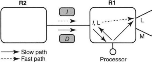
Life gets more exciting if R1 decides to “switch” packets going to D. R1 may decide to do so if, for instance, there is a lot of traffic going to D. In that case, R1 first picks an idle virtual circuit identifier I, places the mapping I → L in its input port hardware, and then sends I back to R2. If R2 now sends packets to D labeled with VCI I to the input port of Rl, the input port looks up the mapping from I to L and switches the packet directly to the output link L without going through the processor.

Of course, R2 can repeat this switching process with the preceding router in the path, and so on. Eventually, IP forwarding can be completely dispensed with in the switched portion of a sequence of flow-switching routers.

Despite its elegance, flow switching seems likely to work poorly in the backbone. This is because backbone flows are short lived and exhibit poor locality. A contrarian opinion is presented in Molinero-Femandez and McKeown [MM02], where the authors argue for the resurrection of flow switching based on TCP connections. They claim that the current use of circuit-switched optical switches to link core routers, the underutilization of backbone links running at 10% of capacity, and increasing optical bandwidths all favor the simplicity of circuit switching at higher speeds.

Both IP and tag switching are techniques to finesse the need for IP lookups by passing information in protocol headers. Like ATM, both schemes rely on passing indices (P10). However, tag switching precomputes the index (P2a) at an earlier time scale (topology change time) than ATM (just before data transfer). On the other hand, in IP switching the indices are computed on demand (P2c, lazy evaluation) after the data begins to flow. However, neither tag nor IP switching completely avoids prefix lookups, and each adds a complex protocol. We now look afresh at the supposed complexity of IP lookups.

11.3 NONALGORITHMIC TECHNIQUES FOR PREFIX MATCHING

In this section, we consider two other systems techniques for prefix lookups that do not rely on algorithmic methods: caching and ternary CAMs. Caching relies on locality in address references, while CAMs rely on hardware parallelism.

11.4 UNIBIT TRIES

It is helpful to start a survey of algorithmic techniques (P15) for prefix lookup with the simplest technique: a unibit trie. Consider the sample prefix database of Figure 11.6. This database will be used to illustrate many of the algorithmic solutions in this chapter. It contains nine prefixes, called P1 to P9, with the bit strings shown in the figure.

In practice, there is a next hop associated with each prefix omitted from the figure. To avoid clutter, prefix names are used to denote the next hops. Thus in the figure, an address D that starts with 1 followed by a string of 31 zeroes will match P6, P7, and P8. The longest match is P7.

Figure 11.7 shows a unibit trie for the sample database of Figure 11.6. A unibit trie is a tree in which each node is an array containing a 0-pointer and a 1-pointer. At the root all prefixes that start with 0 are stored in the subtrie pointed to by the 0-pointer and all prefixes that start with a 1 are stored in the subtrie pointed to by the 1-pointer.

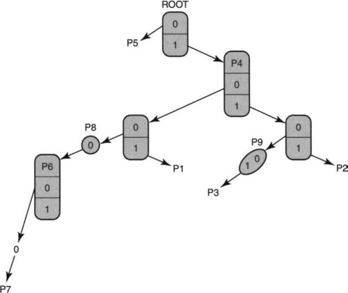
Each subtrie is then constructed recursively in a similar fashion using the remaining bits of the prefixes allocated to the subtrie. For example, in Figure 11.7 notice that P1 = 101 is stored in a path traced by following a 1-pointer at the root, a 0-pointer at the right child of the root, and a 1-pointer at the next node in the path.

There are two other fine points to note. In some cases, a prefix may be a substring of another prefix. For example, P4 = 1* is a substring of P2 = 111*. In that case, the smaller string, P4, is stored inside a trie node on the path to the longer string. For example, P4 is stored at the right child to the root; note that the path to this right child is the string 1, which is the same as P4.

Finally, in the case of a prefix such as P3 = 11001, after we follow the first three bits, we might naively expect to find a string of nodes corresponding to the last two bits. However, since no other prefixes share more than the first 3 bits with P3, these nodes would only contain one pointer apiece. Such a string of trie nodes with only one pointer each is a called a one-way branch.

Clearly one-way branches can greatly increase wasted storage by using whole nodes (containing at least two pointers) when only a single bit suffices. (The exercises will help you quantify the amount of wasted storage.) A simple technique to remove this obvious waste (P1) is to compress the one-way branches

In Figure 11.7, this is done by using a text string (i.e. “01”) to represent the pointers that would have been followed in the one-way branch. Thus in Figure 11.7, two trie nodes (containing two pointers apiece) in the path to P3 have been replaced by a single text string of 2 bits. Clearly, no information has been lost by this transformation. (As an exercise, determine if there is another path in the trie that can similarly be compressed.)

To search for the longest matching prefix of a destination address D, the bits of D are used to trace a path through the trie. The path starts with the root and continues until search fails by ending at an empty pointer or at a text string that does not completely match. While following the path, the algorithm keeps track of the last prefix encountered at a node in the path. When search fails, this is the longest matching prefix that is returned.

For example, if D begins with 1110, the algorithm starts by following the 1-pointer at the root to arrive at the node containing P4. The algorithm remembers P4 and uses the next bit of D (a 1) to follow the 1-pointer to the next node. At this node, the algorithm follows the 1-pointer to arrive at P2. When the algorithm arrives at P2, it overwrites the previously stored value (P4) by the newer prefix found (P2). At this point, search terminates, because P2 has no outgoing pointers.

On the other hand, consider doing a search for a destination D′ whose first 5 bits are 11000. Once again, the first 1 bit is used to reach the node containing P4. P4 is remembered as the last prefix encountered, and the 1 pointer is followed to reach the rightmost node at height 2.

The algorithm now follows the third bit in D′ (a 0) to the text string node containing “01.” Thus we remember P9 as the last prefix encountered. The fourth bit of D′ is a 0, which matches the first bit of “01.” However, the fifth bit of D′ is a 0 (and not a 1 as in the second bit of “01”). Thus the search terminates with P9 as the longest matching prefix.

The literature on tries [Knu73] does not use text strings to compress one-way branches as in Figure 11.7. Instead, the classical scheme, called a Patricia trie, uses a skip count. This count records the number of bits in the corresponding text string, not the bits themselves. For example, the text string node “01” in our example would be replaced with the skip count “2” in a Patricia trie.

This works fine as long as the Patricia trie is used for exact matches, which is what they were used for originally. When search reaches a skip count node, it skips the appropriate number of bits and follows the pointer of the skip count node to continue the search. Since bits that are skipped are not compared for a match, Patricia requires that a complete comparison between the searched key and the entry found by Patricia be done at the end of the search.

Unfortunately, this works very badly with prefix matching, an application that Patricia tries were not designed to handle in the first place. For example, in searching for D′, whose first 5 bits are 11000 in the Patricia equivalent of Figure 11.7, search would skip the last two bits and get to P3. At this point, the comparison will find that P3 does not match D′.

When this happens, a search in a Patricia trie has to backtrack and go back up the trie searching for a possible shorter match. In this example, it may appear that search could have remembered P4. But if P4 was also encountered on a path that contains skip count nodes, the algorithm cannot even be sure of P4. Thus it must backtrack to check if P4 is correct.

Unfortunately, the BSD implementation of IP forwarding [WS95] decided to use Patricia tries as a basis for best matching prefix. Thus the BSD implementation used skip counts; the implementation also stored prefixes by padding them with zeroes. Prefixes were also stored at the leaves of the trie, instead of within nodes as shown in Figure 11.7. The result is that prefix matching can, in the worst case, result in backtracking up the trie for a worst case of 64 memory accesses (32 down the tree and 32 up).

Given the simple alternative of using text strings to avoid backtracking, doing skip counts is a bad idea. In essence, this is because the skip count transformation does not preserve information, while the text string transformation does. However, because of the enormous influence of BSD, a number of vendors and even other algorithms (e.g., Ref. NK98) have used skip counts in their implementations.

11.5 MULTIBIT TRIES

Most large memories use DRAM. DRAM has a large latency (around 60 nsec) when compared to register access times (2–5 nsec). Since a unibit trie may have to make 32 accesses for a 32-bit prefix, the worst-case search time of a unibit trie is at least 32 * 60 = 1.92 μ sec. This clearly motivates multibit trie search.

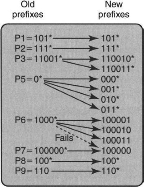
To search a trie in strides of 4 bits, the main problem is dealing with prefixes like 10101* (length 5), whose lengths are not a multiple of the chosen stride length, 4. If we search 4 bits at a time, how can we ensure that we do not miss prefixes like 10101*? Controlled prefix expansion solves this problem by transforming an existing prefix database into a new database with fewer prefix lengths but with potentially more prefixes. By eliminating all lengths that are not multiples of the chosen stride length, expansion allows faster multibit trie search, at the cost of increased database size.

For example, removing odd prefix lengths reduces the number of prefix lengths from 32 to 16 and would allow trie search 2 bits at a time. To remove a prefix like 101* of length 3, observe that 101* represents addresses that begin with 101, which in turn represents addresses that begin with 1010* or 1011*. Thus 101* (of length 3) can be replaced by two prefixes of length 4 (1010* and 1011*), both of which inherit the next hop forwarding entries of 101*.

However, the expanded prefixes may collide with an existing prefix at the new length. In that case, the expanded prefix is removed. The existing prefix is given priority because it was originally of longer length.

In essence, expansion trades memory for time (P4b). The same idea can be used to remove any chosen set of lengths except length 32. Since trie search speed depends linearly on the number of lengths, expansion reduces search time.

Consider the sample prefix database shown in Figure 11.6, which has nine prefixes, P1 to P9. The same database is repeated on the left of Figure 11.8. The database on the right of Figure 11.8 is an equivalent database, constructed by expanding the original database to contain prefixes of lengths 3 and 6 only. Notice that of the four expansions of P6 = 1000* to 6 bits, one collides with P7 = 100000* and is thus removed.

11.5.1 Fixed-Stride Tries

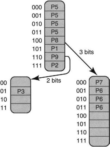
Figure 11.9 shows a trie for the same database as Figure 11.8, using expanded tries with a fixed stride length of 3. Thus each trie node uses 3 bits. The replicated entries within trie nodes in Figure 11.9 correspond exactly to the expanded prefixes on the right of Figure 11.8. For example, P6 in Figure 11.8 has three expansions (100001, 100010, 100011).

These three expanded prefixes are pointed to by the 100 pointer in the root node of Figure 11.9 (because all three expanded prefixes start with 100) and are stored in the 001, 010, and 011 entries of the right child of the root node. Notice also that the entry 100 in the root node has a stored prefix P8 (besides the pointer pointing to P6’s expansions), because P8 = 100* is itself an expanded prefix.

Thus each trie node element is a record containing two entries: a stored prefix and a pointer. Trie search proceeds 3 bits at a time. Each time a pointer is followed, the algorithm remembers the stored prefix (if any). When search terminates at an empty pointer, the last stored prefix in the path is returned.

For example, if address D begins with 1110, search for D starts at the 111 entry at the root node, which has no outgoing pointer but a stored prefix (P2). Thus search for D terminates with P2. A search for an address that starts with 100000 follows the 100 pointer in the root (and remembers P8). This leads to the node on the lower right, where the 000 entry has no outgoing pointer but a stored prefix (P7). The search terminates with result P7. Both the pointer and stored prefix can be retrieved in one memory access using wide memories (P5b).

A special case of fixed-stride tries, described in Gupta et al. [GLM98], uses fixed strides of 24, 4, and 4. The authors observe that DRAMs with more than 2²⁴ locations are becoming available, making even 24-bit strides feasible.

11.5.2 Variable-Stride Tries

In Figure 11.9, the leftmost leaf node needs to store the expansions of P3 = 11001*, while the rightmost leaf node needs to store P6 (1000*) and P7 (100000*). Thus, because of P7, the rightmost leaf node needs to examine 3 bits. However, there is no reason for the leftmost leaf node to examine more than 2 bits because P3 contains only 5 bits, and the root stride is 3 bits. There is an extra degree of freedom that can be optimized (P13).

In a variable-stride trie, the number of bits examined by each trie node can vary, even for nodes at the same level. To do so, the stride of a trie node is encoded with the pointer to the node. Figure 11.9 can be transformed into a variable-stride trie (Figure 11.10) by replacing the leftmost node with a four-element array and encoding length 2 with the pointer to the leftmost node. The stride encoding costs 5 bits. However, the variable stride trie of Figure 11.10 has four fewer array entries than the trie of Figure 11.9.

Our example motivates the problem of picking strides to minimize the total amount of trie memory. Since expansion trades memory for time, why not minimize the memory needed by optimizing a degree of freedom (P13), the strides used at each node? To pick the variable strides, the designer first specifies the worst-case number of memory accesses. For example, with 40-byte packets at 1-Gbps and 80-nsec DRAM, we have a time budget of 320 nsec, which allows only four memory accesses. This constrains the maximum number of nodes in any search path (four in our example).

Given this fixed height, the strides can be chosen to minimize storage. This can be done using dynamic programming [SV99] in a few seconds, even for large databases of 150,000 prefixes. A degree of freedom (the strides) is optimized to minimize the memory used for a given worst-case tree height.

A trie is said to be optimal for height h and a database D if the trie has the smallest storage among all variable-stride tries for database D, whose height is no more than h. It is easy to prove (see exercises) that the trie of Figure 11.10 is optimal for the database on the left of Figure 11.8 and height 2.

The general problem of picking an optimal stride trie can be solved recursively (Figure 11.11). Assume the tree height must be h. The algorithm first picks a root with stride s. The y = 2^s possible pointers in the root can lead to y nonempty subtries T₁,… T_y. If the s-bit pointer p_i leads to subtrie T_i, then all prefixes in the original database D that start with p_i must be stored in T_i. Call this set of prefixes D_i.

Suppose we could recursively find the optimal T_i for height h – 1 and database D_i. Having used up one memory access at the root node, there are only h – 1 memory accesses left to navigate each subtrie T_i. Let C_i, denote the storage cost required, counted in array locations, for the optimal T_i. Then for a fixed root stride s, the cost of the resulting optimal trie C(s) is 2^s (cost of root node in array locations) plus ${\displaystyle {\sum }_{i=1}^y{C}_i}$. Thus the optimal value of the initial stride is the value of s, where 1 ≤ s ≤ 32, that minimizes C(s).

A naive use of recursion leads to repeated subproblems. To avoid repeated subproblems, the algorithm first constructs an auxiliary 1-bit trie. Notice that any subtrie T_i in Figure 11.11 must be a subtrie N of the 1 -bit trie. Then the algorithm uses dynamic programming to construct the optimal cost and trie strides for each subtrie N in the original 1-bit trie for all values of height from 1 to h, building bottom-up from the smallest-height subtries to the largest-height subtries. The final result is the optimal strides for the root (of the 1-bit subtrie) with height h. Details are described in Srinivasan and Varghese [SV99].

The final complexity of the algorithm is easily seen to be O(N * W² * h), where N is the number of original prefixes in the original database, W is the width of the destination address, and h is the desired worst-case height. This is because there are N * W subtries in the 1-bit trie, each of which must be solved for heights that range from 1 to h, and each solution requires a minimization across at most W possible choices for the initial stride s. Note that the complexity is linear in N (the largest number, around 150,000 at the time of writing) and h (which should be small, at most 8), but quadratic in the address width (currently 32). In practice, the quadratic dependence on address width is not a major factor.

For example, Srinivasan and Varghese [SV99] show that using a height of 4, the optimized Mae–East database required 423 KB of storage, compared to 2003 KB for the unoptimized version. The unoptimized version uses the “natural” stride lengths 8, 8, 8, 8. The dynamic program took 1.6 seconds to run on a 300-MHz Pentium Pro. The dynamic program is even simpler for fixed-stride tries and takes only 1 msec to run. However, the use of fixed strides requires 737 KB instead of 423 KB.

Clearly, 1.6 seconds is much too long to let the dynamic program be run for every update and still allow millisecond updates [LMJ97]. However, backbone instabilities are caused by pathologies in which the same set of prefixes S are repeatedly inserted and deleted by a router that is temporarily swamped [LMJ97]). Since we had to allocate memory for the full set, including S, anyway, the fact that the trie is suboptimal in its use of memory when S is deleted is irrelevant. On the other hand, the rate at which new prefixes get added or deleted by managers seems more likely to be on the order of days. Thus a dynamic program that takes several seconds to run every day seems reasonable and will not unduly affect worst-case insertion and deletion times while still allowing reasonably optimal tries.

11.6 LEVEL-COMPRESSED (LC) TRIES

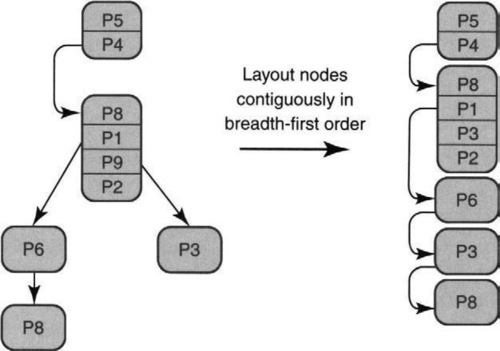
An LC trie [NK98] is a variable-stride trie in which every trie node contains no empty entries. An LC-trie is built by first finding the largest-root stride that allows no empty entries and then recursively repeating this procedure on the child subtries. An example of this procedure is shown in Figure 11.12, starting with a 1-bit trie on the left and resulting in an LC trie on the left. Notice that P4 and P5 form the largest possible full-root subtrie — if the root stride is 2, then the first two array entries will be empty. The motivation, of course, is to avoid empty array elements, to minimize storage.

However, general variable-stride tries are more tunable, allowing memory to be traded for speed. For example, the LC trie representation using a 1997 snapshot of Mae–East has a trie height of 7 and needs 700 KB of memory. By comparison, an optimal variable-stride trie [SV99] has a trie height of 4 using 400 KB. Recall also that the optimal variable-stride calculates the best trie for a given target height and thus would indeed produce the LC trie if the LC trie were optimal for its height.

In its final form, the variable-stride LC trie nodes are laid out in breadth-first order (first the root, then all the trie nodes at the second level from left to right, then third-level nodes, etc.), as shown on the right of Figure 11.13. Each pointer becomes an array offset. The array layout and the requirement for full subtries make updates slow in the worst case. For example, deleting P5 in Figure 11.12 causes a change in the subtrie decomposition. Worse, it causes almost every element in the array representation of Figure 11.13 to be moved upward.

11.7 Lulea-Compressed Tries

Though LC tries and variable-stride tries attempt to compress multibit tries by varying the stride at each node, both schemes have problems. While the use of full arrays allows LC tries not to waste any memory because of empty array locations, it also increases the height of the trie, which cannot then be tuned. On the other hand, variable-stride tries can be tuned to have short height, at the cost of wasted memory because of empty array locations in trie nodes. The Lulea approach [DBCP97], which we now describe, is a multibit-trie scheme that uses fixed-stride trie nodes of large stride but uses bitmap compression to reduce storage considerably.

We know that a string with repetitions (e.g., AAAABBAAACCCCC) can be compressed using a bitmap denoting repetition points (i.e., 10001010010000) together with a compressed sequence (i.e., ABAC). Similarly, the root node of Figure 11.9 contains a repeated sequence (P5, P5, P5, P5) caused by expansion.

The Lulea scheme [DBCP97] avoids this obvious waste by compressing repeated information using a bitmap and a compressed sequence without paying a high penalty in search time. For example, this scheme used only 160 KB of memory to store the Mae–East database. This allows the entire database to fit into expensive SRAM or on-chip memory. It does, however, pay a high price in insertion times.

Some expanded trie entries (e.g., the 110 entry at the root of Figure 11.9) have two values, a pointer and a prefix. To make compression easier, the algorithm starts by making each entry have exactly one value by pushing prefix information down to the trie leaves. Since the leaves do not have a pointer, we have only next-hop information at leaves and only pointers at nonleaf nodes. This process is called leaf pushing.

For example, to avoid the extra stored prefix in the 110 entry of the root node of Figure 11.9, the P9 stored prefix is pushed to all the entries in the leftmost trie node, with the exception of the 010 and 011 entries (both of which continue to contain P3). Similarly, the P8 stored prefix in the 100 root node entry is pushed down to the 100, 101, 110, and 111 entries of the rightmost trie node. Once this is done, each node entry contains either a stored prefix or a pointer but not both.

The Lulea scheme starts with a conceptual leaf-pushed expanded trie and replaces consecutive identical elements with a single value. A node bitmap (with 0’s corresponding to removed positions) is used to allow fast indexing on the compressed nodes.

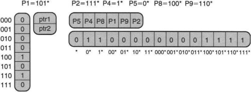
Consider the root node in Figure 11.9. After leaf pushing, the root has the sequence P5, P5, P5, P5, ptr1, P1, ptr2, P2 (ptrl is a pointer to the trie node containing P6 and P7, and ptr2 is a pointer to the node containing P3). After replacing consecutive values with the first value, we get P5, -, -, -, ptr1, P1, ptr2, P2, as shown in the middle frame of Figure 11.14. The rightmost frame show the final result, with a bitmap indicating removed positions (10001111) and a compressed list (P5, ptrl, P1, ptr2, P2).

If there are N original prefixes and pointers within an original (unexpanded) trie node, the number of entries within the compressed node can be shown never to be more than 2N + 1. Intuitively, this is because N prefixes partition the address space into at most 2N + 1 disjoint subranges and each subrange requires at most one compressed node entry.

Search uses the number of bits specified by the stride to index into the current trie node, starting with the root and continuing until a null pointer is encountered. However, while following pointers, an uncompressed index must be mapped to an index into the compressed node. This mapping is accomplished by counting bits within the node bitmap.

Consider the data structure on the right of Figure 11.14 and a search for an address that starts with 100111. If we were dealing with just the uncompressed node on the left of Figure 11.14, we could use 100 to index into the fifth array element to get ptr1. However, we must now obtain the same information from the compressed-node representation on the right of Figure 11.14.

Instead, we use the first three bits (100) to index into the root-node bitmap. Since this is the second bit set (the algorithm needs to count the bits set before a given bit), the algorithm indexes into the second element of the compressed node. This produces a pointer ptrl to the rightmost trie node. Next, imagine the rightmost leaf node of Figure 11.9 (after leaf pushing) also compressed in the same way. The node contains the sequence P7, P6, P6, P6, P8, P8, P8, P8. Thus the corresponding bitmap is 11001000, and the compressed sequence is P7, P6, P8.

Thus in the rightmost leaf node, the algorithm uses the next 3 bits (111) of the destination address to index into bit 8. Since this bit is a 0, the search terminates: There is no pointer to follow in the equivalent uncompressed node. However, to retrieve the best matching prefix (if any) at this node, the algorithm must find any prefix stored before this entry.

This would be trivial with expansion because the value P8 would have been expanded into the 111 entry; but since the expanded sequence of P8 values has been replaced by a single P8 value in the compressed version, the algorithm has to work harder. Thus the Lulea algorithm counts the number of bits set before position 8 (which happens to be 3) and then indexes into the third element of the compressed sequence. This gives the correct result, P8.

The Lulea paper [DBCP97] describes a trie that uses fixed strides of 16, 8, and 8. But how can the algorithm efficiently count the bits set in a large bitmap, for example, a 16-bit stride uses 64K bits? Before you read on, try to answer this question using principles P12 (adding state for speed) and P2a (precomputation).

To speed up counting set bits, the algorithm accompanies each bitmap with a summary array that contains a cumulative count (precomputed) of the number of set bits associated with fixed-size chunks of the bit map. Using 64-bit chunks, the summary array takes negligible storage. Counting the bits set up to position i now takes two steps. First, access the summary array at position j, where j is the chunk containing bit i. Then access chunk j and count the bits in chunk j up to position i. The sum of the two values gives the count.

While the Lulea paper uses 64-bit chunks, the example in Figure 11.15 uses 8-bit chunks. The large bitmap is shown from left to right, starting with 10001001, as the second array from the top. Each 8-bit chunk has a summary count that is shown as an array above the bitmap. The summary count for chunk i counts the cumulative bits in the previous chunks of the bitmap (not including chunk i).

Thus the first chunk has count 0, the second has count 3 (because 10001001 has three bits set), and the third has count 5 (because 10001001 has two bits set, which added to the previous chunk’s value of 3 gives a cumulative count of 5).

Consider searching for the bits set up to position X in Figure 11.15, where X can be written as J011. Clearly, X belongs to chunk J. The algorithm first looks up the summary count array to retrieve numSet[J]. This yields the number of bits set up to but not including chunk J. The algorithm then retrieves chunk J itself (10011000) and counts the number of bits set until the third position of chunk J. Since the first three bits of chunk J are 100, this yields the value 1. Finally, the desired overall bit count is numSet[J] + 1.

Notice that the choice of the chunk size is a trade-off between memory size and speed. Making a chunk equal to the size of the bitmap will make counting very slow. On the other hand, making a chunk equal to a bit will require more storage than the original trie node! Choosing a 64-bit chunk size makes the summary array size only 1/64 the size of the original node, but this requires counting the bits set within a 64-bit chunk. Counting can easily be done using special instructions in software and via combinational logic in hardware.

Thus search of a node requires first indexing into the summary table, then indexing into the corresponding bitmap chunk to compute the offset into the compressed node, and finally retrieving the element from the compressed node. This can take three memory references per node, which can be quite slow.

The final Lulea scheme also compresses entries based on their next-hop values (entries with the same next-hop values can be considered the same even though they match different prefixes). Overall the Lulea scheme has very compact storage. Using an early (1997) snap-shot of the Mae–East database of around 40,000 entries, the Lulea paper [DBCP97] reports compressing the entire database to around 160 KB, which is roughly 32-bits per prefix.

This is a very small number, given that one expects to use at least one 20-bit pointer per prefix in the database. The compact storage is a great advantage because it allows the prefix database to potentially fit into limited on-chip SRAM, a crucial factor in allowing prefix lookups to scale to OC-768 speeds.

Despite compact storage, the Lulea scheme has two disadvantages. First, counting bits requires at least one extra memory reference per node. Second, leaf pushing makes worst-case insertion times large. A prefix added to a root node can cause information to be pushed to thousands of leaves. The full tree bitmap scheme, which we study next, overcomes these problem by abandoning leaf pushing and using two bitmaps per node.

11.8 TREE BITMAP

The tree bitmap [EDV] scheme starts with the goal of achieving the same storage and speed as the Lulea scheme, but it adds the goal of fast insertions. While we have argued that fast insertions are not as important as fast lookups, they clearly are desirable. Also, if the only way to handle an insertion or deletion is to rebuild the Lulea-compressed trie, then a router must keep two copies of its routing database, one that is being built and one that is being used for lookups. This can potentially double the storage cost from 32 bits per prefix to 64 bits per prefix. This in turn can halve the number of prefixes that can be supported by a chip that places the entire database in on-chip SRAM.

To obtain fast insertions and hence avoid the need for two copies of the database, the first problem in Lulea that must be handled is the use of leaf pushing. When a prefix of small length is inserted, leaf pushing can result in pushing down the prefix to a large number of leaves, making insertion slow.

11.8.1 Tree Bitmap Ideas

Thus the first and main idea in the tree bitmap scheme is that there be two bitmaps per trie node, one for all the internally stored prefixes and one for the external pointers. Figure 11.16 shows the tree bitmap version of the root node in Figure 11.14.

Recall that in Figure 11.14, the prefixes P8 = 100* and P9 = 110* in the original database are missing from the picture on the left side because they have been pushed down to the leaves to accommodate the two pointers (ptr1, which points to nodes containing longer prefixes such as P6 = 1000*, and ptr2, which points to nodes containing longer prefixes such as P3 = 11001*). This results in the basic Lulea trie node, in which each element contains either a pointer or a prefix but not both. This allows the use of a single bitmap to compress a Lulea node, as shown on the extreme right of Figure 11.14.

By contrast, the same trie node in Figure 11.16 is split into two compressed arrays, each with its own bitmap. The first array, shown vertically, is a pointer array, which contains a bitmap denoting the (two) positions where nonnull pointers exist and a compressed array containing the nonnull pointers, ptr1 and ptr2.

The second array, shown horizontally, is the internal prefix array, which contains a list of all the prefixes within the first 3 bits. The bitmap used for this array is very different from the Lulea encoding and has one bit set for every possible prefix stored within this node. Possible prefixes are listed lexicographically, starting from *, followed by 0* and 1*, and then on to the length-2 prefixes (00*, 01*, 10*, 11*), and finally the length-3 prefixes. Bits are set when the corresponding prefixes occur within the trie node.

Thus in Figure 11.16, the prefixes P8 and P9, which were leaf pushed in Figure 11.14, have been resurrected and now correspond to bits 12 and 14 in the internal prefix bitmap. In general, for an r-bit trie node, there are 2^r+1 – 1 possible prefixes of lengths r or less, which requires the use of a (2^r+1 – 1) bitmap. The scheme gets its name because the internal prefix bitmap represents a trie in a linearized format: Each row of the trie is captured top-down from left to right.

The second idea in the tree bitmap scheme is to keep the trie nodes as small as possible to reduce the required memory access size for a given stride. Thus a trie node is of fixed size and contains only a pointer bitmap, an internal prefix bitmap, and child pointers. But what about the next-hop information associated with any stored prefixes?

The trick is to store the next hops associated with the internal prefixes stored within each trie node in a separate array associated with this trie node. Putting next-hop pointers in a separate result array potentially requires two memory accesses per trie node (one for the trie node and one to fetch the result node for stored prefixes).

However, a simple lazy evaluation strategy (P2b) is not to access the result nodes until search terminates. Upon termination, the algorithm makes a final access to the correct result node. This is the result node that corresponds to the last trie node encountered in the path that contained a valid prefix. This adds only a single memory reference at the end, in addition to the one memory reference required per trie node.

The third idea is to use only one memory access per node, unlike Lulea, which uses at least two memory accesses. Lulea needs two memory accesses per node because it uses large strides of 8 or 16 bits. This increases the bitmap size so much that the only feasible way to count bits is to use an additional chunk array that must be accessed separately. The tree bitmap scheme gets around this by simply using smaller-stride nodes, say, of 4 bits. This makes the bitmaps small enough that the entire node can be accessed by a single wide access (P4a, exploit locality). Combinatorial logic (Chapter 2) can be used to count the bits.

11.9 BINARY SEARCH ON RANGES

So far, all our schemes (unibit tries, expanded tries, LC tries, Lulea tries, tree bitmaps) have been trie variants. Are there other algorithmic paradigms (P15) to the longest-matching-prefix problem? Now, exact matching is a special case of prefix matching. Both binary search and hashing [CLR90] are well-known techniques for exact matching. Thus we should consider generalizing these standard exact-matching techniques to handle prefix matching. In this section, we examine an adaptation of binary search; in the next section, we look at an adaptation of hashing.

In binary search on ranges [LSV98], each prefix is represented as a range, using the start and end of the range. Thus the range endpoints for N prefixes partition the space of addresses into 2N + 1 disjoint intervals. The algorithm [LSV98] uses binary search to find the interval in which a destination address lies. Since each interval corresponds to a unique prefix match, the algorithm precomputes this mapping and stores it with range endpoints. Thus prefix matching takes log₂(2N) memory accesses.

Consider a tiny routing table with only two prefixes, P4 = 1* and P1 = 101*. This is a small subset of the database used in Figure 11.8. Figure 11.17 shows how the binary search data structure is built as a table (left) and as a binary tree (right).

The starting point for this scheme is to consider a prefix as a range of addresses. To keep things simple, imagine that addresses are 4 bits instead of 32 bits. Thus P4 = 1* is the range 1000 to 1111, and P1 = 101* is the range 1000 to 1011. Next, after adding in the range for the entire address space (0000 to 1111), the endpoints of all ranges are sorted into a binary search table, as shown on the left of Figure 11.17.

In Figure 11.17, the range endpoints are drawn vertically on the left. The figure also shows the ranges covered by each of the prefixes. Next, two next-hop entries are associated with each endpoint. The leftmost entry, called the > entry, is the next hop corresponding to addresses that are strictly greater than the endpoint but strictly less than the next range endpoint in sorted order. The rightmost entry, called the = entry, corresponds to addresses that are exactly equal to the endpoint.

For example, it should be clear from the ranges covered by the prefixes that any addresses greater than or equal to 0000 but strictly less than 1000 do not match any prefix. Hence the entries corresponding to 0000 are –, to denote no next hop.³ Similarly, any address greater than or equal to 1000 but strictly less than 1010 must match prefix P4 = 1*.

The only subtle case, which illustrates the need for two separate entries for > and = , is the entry for 1011. If an address is strictly greater than 1011 but strictly less than the next entry, 1111, then the best match is P4. Thus the > pointer is P4. On the other hand, if an address is exactly equal to 1011, its best match is P1. Thus the = pointer is P1.

The entire data structure can be built as a binary search table, where each table entry has three items, consisting of an endpoint, a > next-hop pointer, and a = next-hop pointer. The table has at most 2N entries, because each of N prefixes can insert two endpoints. Thus after the next-hop values are precomputed, the table can be searched in log₂ 2N time using binary search on the endpoint values. Alternatively, the table can be drawn as a binary tree, as shown on the right in Figure 11.17. Each tree node contains the endpoint value and the same two next-hop entries.

The description so far shows that binary search on values can find the longest prefix match after log₂ 2N time. However, the time can be reduced using binary trees of higher radix, such as B-trees. While such trees require wider memory accesses, this is an attractive trade-off for DRAM-based memories, which allow fast access to consecutive memory locations (P4a).

Computational geometry [PS85] offers a data structure called a range tree for finding the narrowest range. Range trees offer fast insertion times as well as fast O(log₂ N) search times. However, there seems to be no easy way to increase the radix of range trees to obtain O(log_M N) search times for M > 2.

As described, this data structure can easily be built in linear time using a stack and an additional trie. It is not hard to see that even with a balanced binary tree (see exercises), adding a short prefix can change the > pointers of a large number of prefixes in the table. A trick to allow fast insertions and deletions in logarithmic time is described in Warkhede et al. [WSV01b],

Binary search on prefix values is somewhat slow when compared to multibit tries. It also uses more memory than compressed trie variants. However, unlike the other trie schemes, all of which are subject to patents, binary search is free of such restrictions. Thus at least a few vendors have implemented this scheme into hardware. In hardware, the use of a wide memory access (to reduce the base of the logarithm) and pipelining (to allow one lookup per memory access) can make this scheme sufficiently fast.

11.10 BINARY SEARCH ON PREFIX LENGTHS

In this section, we adapt another classical exact-match scheme, hashing, to longest prefix matching. Binary search on prefix lengths finds the longest match using log₂ W hashes, where W is the maximum prefix length. This can provide a very scalable solution for 128-bit IPv6 addresses. For 128-bit prefixes, this algorithm takes only seven memory accesses, as opposed to 16 memory accesses using a multibit trie with 8-bit strides. To do so, the algorithm first segregates prefixes by length into separate hash tables. More precisely, it uses an array L of hash tables such that L[i] is a pointer to a hash table containing all prefixes of length i.

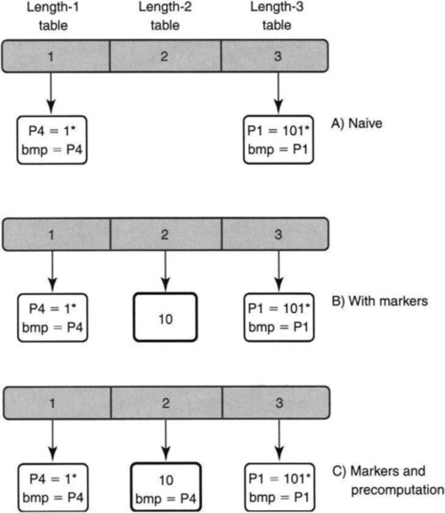
Assume the same tiny routing table, with only two prefixes, P4 = 1* and P1 = 101*, of lengths 1 and 3, respectively, that was used in Figure 11.17. Recall that this is a small subset of Figure 11.8. The array of hash tables is shown horizontally in the top frame (A) of Figure 11.18. The length-1 hash table storing P4 is shown vertically on the left and is pointed to by position 1 in the array; the length-3 hash table storing P1 is shown on the right and is pointed to by position 3 in the array; the length-2 hash table is empty because there are no prefixes of length 2.

Naively, a search for address D would start with the greatest-length hash table l (i.e., 3), would extract the first i bits of D into D_l, and then search the length-l hash table for D_l. If search succeeds, the best match has been found; if not, the algorithm considers the next smaller length (i.e., 2). The algorithm moves in decreasing order among the set of possible prefix lengths until it either finds a match or runs out of lengths.

The naive scheme effectively does linear search among the distinct prefix lengths. The analogy suggests a better algorithm: binary search (P15). However, unlike binary search on prefix ranges, this is binary search on prefix lengths. The difference is major. With 32 lengths, binary search on lengths takes five hashes in the worst case; with 32,000 prefixes, binary search on prefix ranges takes 16 accesses.

Binary search must start at the median prefix length, and each hash must divide the possible prefix lengths in half. A hash search gives only two values: found and not found. If a match is found at length m, then lengths strictly greater than m must be searched for a longer match. Correspondingly, if no match is found, search must continue among prefixes of lengths strictly less than m.

For example, in Figure 11.18, part (A), suppose search begins at the median length-2 hash table for an address that starts with 101. Clearly, the hash search does not find a match. But there is a longer match in the length-3 table. Since only a match makes search move to the right half, an “artificial match,” or marker, must be introduced to force the search to the right half when there is a potentially longer match.

Thus part (B) introduces a bolded marker entry 10, corresponding to the first two bits of prefix P1 = 101, in the length-2 table. In essence, state has been added for speed (P12). The markers allow probe failures in the median to rule out all lengths greater than the median.

Search for an address D that starts with 101 works correctly. Search for 10 in the length-2 table (in Part (B) of Figure 11.18) results in a match; search proceeds to the length-3 table, finds a match with P1, and terminates. In general, a marker for a prefix P must be placed at all lengths that binary search will visit in a search for P. This adds only a logarithmic number of markers. For a prefix of length 32, markers are needed only at lengths 16, 24, 28, and 30.

Unfortunately, the algorithm is still incorrect. While markers lead to potentially longer prefixes, they can also cause search to follow false leads. Consider a search for an address D′ whose first three bits are 100 in part (B) of Figure 11.18. Since the median table contains 10, search in the middle hash table results in a match. This forces the algorithm to search in the third hash table for 100 and to fail. But the correct best matching prefix is at the first hash table — i.e., P4 = 1*. Markers can cause the search to go off on a wild goose chase! On the other hand, a backtracking search of the left half would result in linear time.

To ensure logarithmic time, each marker node M contains a variable M.bmp, where M.bmp is the longest prefix that matches string M. This is precomputed when M is inserted into its hash table. When the algorithm follows marker M and searches for prefixes of lengths greater than M, and if the algorithm fails to find such a longer prefix, then the answer is M.bmp. In essence, the best matching prefix of every marker is precomputed (P2a). This avoids searching all lengths less than the median when a match is obtained with a marker.

The final version of the database containing prefixes P4 and P1 is shown in part (C) of Figure 11.18. A bmp field has been added to the 10 marker that points to the best matching prefix of the string 10 (i.e., P4 = 1*). Thus when the algorithm searches for 100 and finds a match in the median length-2 table, it remembers the value of the corresponding bmp entry P4 before it searches the length-3 table. When the search fails (in the length-3 table), the algorithm returns the bmp field of the last marker encountered (i.e., P4).

A trivial algorithm for building the simple binary search data structure from scratch is as follows. First determine the distinct prefix lengths; this determines the sequence of lengths to search. Then add each prefix P in turn to the hash table corresponding to length(P). For each prefix, also add a marker to all hash tables corresponding to lengths L < length(P) that binary search will visit (if one does not already exist). For each such marker M, use an auxiliary 1-bit trie to determine the best matching prefix of M. Further refinements are described in Waldvogel et al. [WVTP01].

While the search algorithm takes five hash table lookups in the worst case for IPv4, we note that in the expected case most lookups should take two memory accesses. This is because the expected case observation O1 shows that most prefixes are either 16 or 24 bits (at least today). Thus doing binary search at 16 and then 24 will suffice for most prefixes.

The use of hashing makes binary search on prefix lengths somewhat difficult to implement in hardware. However, its scalability to large prefix lengths, such as IPv6 addresses, has made it sufficiently appealing to some vendors.

11.11 MEMORY ALLOCATION IN COMPRESSED SCHEMES

With the exception of binary search and fixed-stride multibit tries, many of the schemes described in this chapter need to allocate memory in different sizes. Thus if a compressed trie node grows from two to three memory words, the insertion algorithm must deallocate the old node of size 2 and allocate a new node of size 3. Memory allocation in operating systems is a somewhat heuristic affair, using algorithms, such as best-fit and worst-fit, that do not guarantee worst-case properties.

In fact all standard memory allocators can have a worst-case fragmentation ratio that is very bad. It is possible for allocates and deallocates to conspire to break up memory into a patchwork of holes and small allocated blocks. Specifically, if Max is the size of the largest memory allocation request, the worst-case scenario occurs when all holes are of size Max – 1 and all allocated blocks are of size 1. This can occur by allocating all of memory using requests of size 1, followed by the appropriate deallocations. The net result is that only $\frac{1}{Max}$ of memory is guaranteed to be used, because all future requests may be of size Max.

The allocator’s use of memory translates directly into the maximum number of prefixes that a lookup chip can support. Suppose that — ignoring the allocator — one can show that 20 MB of on-chip memory can be used to support 640,000 prefixes in the worst case. If one takes the allocator into account and Max = 32, the chip can guarantee supporting only 20,000 prefixes!

Matters are not helped by the fact that CAM vendors at the time of writing were advertising a worst-case number of 100,000 prefixes, with 10-nsec search times and microsecond update times. Thus, given that algorithmic solutions to prefix lookup often compress data structures to fit into SRAM, algorithmic solutions must also design memory allocators that are fast and that minimally fragment memory.

There is an old result [Rob74] that says that no allocator that does not compact memory can have a utilization ratio better than $\frac{1}{{\log }_{2}Max}$. For example, this is 20% for Max = 32. Since this is unacceptable, algorithmic solutions involving compressed data structures must use compaction. Compaction means moving allocated blocks around to increase the size of holes.

Compaction is hardly ever used in operating systems, for the following reason. If you move a piece of memory M, you must correct all pointers that point to M. Fortunately, most lookup structures are trees, in which any node is pointed to by at most one other node. By maintaining a parent pointer for every tree node, nodes that point to a tree node M can be suitably corrected when M is relocated. Fortunately, the parent pointer is needed only for updates and not for search. Thus the parent pointers can be stored in an off-chip copy of the database used for updates in the route processor, without consuming precious on-chip SRAM.

Even after this problem is solved, one needs a simple algorithm that decides when to compact a piece of memory. The existing literature on compaction is in the context of garbage collection (e.g., Refs. Wil92, LB96) and tends to use global compactors that scan through all of memory in one compaction cycle. To bound insertion times, one needs some form of local compactor that compacts only a small amount of memory around the region affected by an update.

11.12 LOOKUP-CHIP MODEL

Given speed increases to OC-768 speeds, lookup schemes will probably be implemented on chips rather than on network processors, at least for the very highest speeds. Figure 11.19 describes a model of a lookup chip that does search and update. The chip has a Search and an Update process, both of which access a common SRAM memory that is either on or off chip (or both). The Update process allows incremental updates and (potentially) does a memory allocation/deallocation and a small amount of local compaction for every update.

The actual updates can be done either completely on chip, partially in software, or completely in software. If a semiconductor company wishes to sell a lookup chip using a complex update algorithm (e.g., for compressed schemes), it may be wiser also to provide an update algorithm in hardware. If the lookup chip is part of a forwarding engine, however, it may be simpler to relegate the update process completely to a separate CPU on the line card.

Each access to SRAM can be fairly wide if needed, even up to 1000 bits. This is quite feasible today using a wide bus. The search and update logic can easily process 1000 bits in parallel in one memory cycle time. Recall that wide word accesses can help — for example, in the tree bitmap and binary search on values schemes — to reduce search times.

Search and Update use time multiplexing to share access to the common SRAM that stores the lookup database. Thus the Search process is allowed S consecutive accesses to memory, and then the Update process is allowed K accesses to memory. If S is 20 and K is 2, this allows Update to steal a few cycles from Search while slowing down Search throughput by only a small fraction. Note that this increases the latency of Search by K memory accesses in the worst case; however, since the Search process is likely to be pipelined, this can be considered a small additional pipeline delay.

The chip has pins to receive inputs for Search (e.g., keys) and Update (e.g., update type, key, result) and can return search outputs (e.g., result). The model can be instantiated for various types of lookups, including IP lookups (e.g., 32-bit IP addresses as keys and next hops as results), bridge lookups (48-bit MAC addresses as keys and output ports as results), and classification (e.g., packet headers as keys and matching rules as results).

Each addition or deletion of a key can result in a call to deallocate a block and to allocate a different-size block. Each allocate request can be in any range from 1 to Max memory words. There is a total of M words that can be allocated. The actual memory can be either off chip, on chip, or both. Clearly, even off-chip solutions will cache the first levels of any lookup tree on chip. On-chip memory is attractive because of its speed and cost. Unfortunately, on-chip memory was limited by current processes to around 32 Mbits at the time of writing. This makes it difficult to support databases of 1 million prefixes.

Internally, the chip will very likely be heavily pipelined. The lookup data structure is partitioned into several pieces, each of which is concurrently worked on by separate stages of logic. Thus the SRAM will likely be broken into several smaller SRAMs that can be accessed independently by each pipeline stage.

There is a problem [SV00] with statically partitioning SRAM between pipeline stages, because memory needs for each stage can vary as prefixes are inserted and deleted. One possible solution is to break the single SRAM into a fairly large number of smaller SRAMs that can be dynamically allocated to the stages via a partial crossbar switch. However, designing such a crossbar at very high speeds is not easy.

All the schemes described in this chapter can be pipelined because they are all fundamentally based on trees. All nodes at the same depth in a tree can be allocated to the same pipeline stage.

11.13 CONCLUSIONS

It is important to gain some perspective after the large number of isolated lookup variants described in this chapter. Thus we conclude with a summary of the state of the art in lookups, and a survey of the common principles used in their design.

State of the Art in Lookups: Lookup schemes are coming under severe pressure in core routers as both table sizes (up to 1 million prefixes) and speed (up to 40 Gbps) ratchet upwards. MPLS, once thought to be a way to finesse lookups, is now mostly used to avoid packet classification for traffic engineering purposes. CAMs are nibbling away at even the core router space, but the large cost, power, and board real estate issues of large CAMs remain issues. Thus many core router vendors are still using and designing algorithmic schemes for lookups.

Oddly enough, even after the algorithmic riches explored in this chapter, simple unibit tries together with SRAM and pipelining work well, even at 40-Gbps speeds. This is because path-compressed unibit tries are relatively compact; their slow search times can be offset by a pipeline together with an initial array lookup. Recall, however, that pipelining is trickier than it looks because of the need to partition memory among stages.

At slower speeds of up to 10 Gbps, simple multibit tries using controlled prefix expansion work well with DRAM. While DRAM is slow, it is plentiful and cheap. The use of RAMBUSlike technologies can allow lookup pipelining even with network processors. The simplicity of this scheme has proved attractive to a number of vendors.

Some vendors even use binary search on values; its speed and memory use are reasonable, especially with B-trees with wide memories to reduce tree height. The binary-search-on-ranges scheme is also unencumbered with patents.

At the highest speeds, the number of pipeline stages can be reduced from 20 to 5 using multibit tries. However, multibit tries must be compressed to fit into limited SRAM, when on or off chip. While Lulea’s compression is remarkable, it appears that the algorithm can be used today only via custom solutions sold by a company called Effnet. The Lulea scheme also has slow updates. By contrast, the tree bitmap scheme has fast updates and can be tailored to a wide variety of hardware settings [EDV]. However, there may be patents that restrict the use of tree bitmap as well. It is used today in Cisco’s CRS-1 Router.

Finally, binary search on prefix lengths is attractive because of its scaling properties to large address lengths. Unfortunately, its use of hashing makes it hard to guarantee lookup times. Similarly, the slow deployment of IPv6 and multicast, both of which increase the importance of long address lookup, have made this scheme less attractive. It is, however, used by a few vendors in software implementations. It may be a contender in the future.

The bottom line is that algorithmic solutions together with pipelining can scale with link speeds as long as SRAM speeds scale to match packet arrival times. All the schemes studied in this chapter can be pipelined to provide one lookup per memory access time. The choice between CAMs and algorithmic schemes will continue to be hard to quantify and will probably be made on an ad hoc basis for each product.

However, fundamentally, if compressed trie schemes can use less than 32 bits per prefix, compressed tries appear to use fewer transistors and less power than CAMs. This is because in a CAM the lookup logic is distributed in each of N memory cells, whereas in an algorithmic solution the lookup logic, albeit more complicated, is distributed among a small, constant number of stages. A careful VLSI scaling analysis of these two approaches would be very useful.

Underlying Principles: Although this is a chapter about lookups and thinking about lookups requires paying attention to current market trends, it is important not to forget that this is a book about underlying principles. It is plausible that routers in the misty future may use all-optical switches and all-optical processing, even for lookups. In that case, the specific algorithms described in this chapter may be discarded; but perhaps the underlying design principles will remain.

Although the schemes described in this chapter require some algorithmic thinking, they also employ many of the other principles we have stressed. The schemes make heavy use of precomputation, which trades slower insert/delete times for fast search times. The schemes also exploit hardware features such as wide memories, distinguish fast and slow memories, trade memory for time, and optimize the degrees of freedom in a given design. Figure 11.1 summarizes the schemes and the principles used in them.

Finally, this chapter cannot hope to do justice to all the interesting IP lookup schemes that have been published in the academic and patent literature. You can look it up.

11.14 EXERCISES

1. Caching Prefixes: Suppose we have the prefixes 10*, 100*, and 1001*. Hugh Hopeful would like to cache prefixes instead of entire 32-bit addresses. Hugh’s scheme keeps a set of prefixes in the cache (fast memory), in addition to the complete set of prefixes in slow memory. Hugh’s scheme first does a best-matching-prefix search in the cache; if a matching prefix is found, the next hop of the prefix is used. If no matching prefix is found, a best-matching-prefix search is done for the entire database and the resulting prefix cached. Periodically, prefixes that have not been matched for a while are flushed from the cache. Alyssa P. Hacker quickly gives Hugh a counterexample to show him that his scheme is flawed and that caching prefixes is tricky (if not impossible). Can you?

2. Encoding Prefixes in a Constant Length: We said in the text that encoding prefixes like 10*, 100*, and 1000* in a fixed length could not be done by padding prefixes with zeroes. It clearly can be done by padding with zeroes and adding an encoding of the prefix length. We want to study a more efficient method.

• How many possible prefixes on 32 bits can there be?

• Show how to encode all such prefixes using a fixed length of 33 bits. Make sure that 10*, 100*, and 1000* encode to different values.

• Can you use this fixed-length encoding of prefixes to have the multiple hash tables used in Section 11.10 be packed into a single hash table? Why might this help to decrease the chances of hash collisions for a given memory size?

3. Quantifying the Benefits of Compressing One-Way Branches:

• For a unibit trie that does not compress one-way branches, show that the maximum number of trie nodes can be O(N · W), where N is the number of prefixes and W is the maximum prefix length. (Hint: Generate a trie that uses log₂ N levels to generate N nodes, and then hang a long string of N – W nodes from each of the N nodes.)

• Show that a unibit trie with text strings to compress one-way branches can have at most 2N trie nodes and 2N text strings.

• Extend your analysis to multibit trie nodes with a fixed stride. How would you implement text string compression in such tries?

4. Controlled Prefix Expansion: Code up an efficient algorithm that expands a set of prefixes to any target set of lengths L₁,…, L_k. Check your algorithm using the sample database of Figure 11.8. What is the complexity of your algorithm?

5. Optimal Variable-Stride Trie: Prove that the varied-stride trie of Figure 11.10 is optimal for a trie height of 2. Use the recursive formulation shown in the text.

6. Reducing Memory References in Lulea: The naive approach to counting bits shown in Figure 11.15 should take three memory references (to access numSet, to read the appropriate chunk of the bitmap, and to access the compressed trie node for the actual information.) Show how to use P4a to combine the first two accesses into a single access.

7. Next Node versus Leaf Pushing in Lulea: Before we applied Lulea compression, we first leaf pushed the expanded trie of Figure 11.9. The motivation was to make every entry either a pointer or a prefix but not both. Suppose we have a special prefix entry at the top of every trie node; if any entry in a trie node has pointer p and prefix P, we push P to the top of the node pointed to by p. Thus we would push the prefix P8 in the 100 entry of the root of Figure 11.9 to the top of the rightmost trie node.

• We cited leaf pushing as one of the reasons for slow insertion times in the Lulea scheme. Does next-node pushing allow incremental insertion for the Lulea scheme?

• How would you modify trie search to take into account the fact that prefixes can be stored at the top of (potentially large) trie nodes? How would this increase the search time (in memory accesses) of the Lulea scheme?

8. CAM Node Compression: Instead of using the Lulea scheme for compression, we could just store all the prefixes within a trie node without expansion. If we use small trie nodes (3- or 4-bit strides), a chip can potentially read all the entries in a node and internally do a comparison to find the best-matching prefix within the node. Describe the details of such a scheme.

9. Tree Bitmap Algorithm: The tree bitmap algorithm described in the text requires rooting through the internal prefix bitmap to decide if there was a matching prefix at a trie node N before moving on. This requires a greater access width (to access the internal prefix bitmaps) and more time. Consider adding state to the next node in the search path (P12) and one more final memory access to avoid this overhead.

10. Multicolumn Binary Search: In Chapter 4 we saw how to efficiently use binary search when the identifiers were wide. Explain how to combine this idea with that of binary search on prefixes explained in this chapter in order to do IPv6 lookups (up to 128-bit prefixes). How does this scheme compare with the other schemes in terms of lookup performance for IPv6?

11. Binary Search with Fast Incremental Updates: (This is difficult.) Find a way to remove all the problems of updates to binary search. The key problem is that if a large prefix range R contains lots of disjoint prefix ranges R₁,… R_k, then the spaces between the ranges R_k must be precomputed to map to R. If we now add a new prefix range, R′. that is contained in R but still contains R₁ through R_k, then all the spaces between the ranges R_k must be changed to map to the new range, R′. Since k can be O(n), this could lead to a O(n) update. Try to avoid this problem by storing the binary search database as a tree and storing information about precomputed prefixes that cover the space between ranges as high as possible in the tree, as opposed to storing in the leaves. Details can be found in Warkhede et al. [WSV01b].

12. Counterexamples for Binary Search on Prefix Lengths: Even in industry, it is often useful to show by counter example that worst cases can actually exist. This ensures that we are not doing unnecessary work, and it also silences people who say that the worst case will never be too bad. Imagine that Hugh Hopeful is working for the same startup building an IP lookup chip. The company is now considering using binary search on prefix lengths.

• Suppose we use only markers and no precomputation. This would make insertion a lot faster. Hugh Hopeful suggests that backtracking can only lead to a logarithmic number of extra accesses. Find an example that leads to linear time.

• Hugh Hopeful finds that in practice real databases add only 25% extra marker storage, much less than the log₂ W multiplicative factor that we claimed. This is important because he would like to boast of a larger number of prefixes that his chip can handle for the given amount of memory. Give a worst-case example to show that we can add log₂ W entries per marker.

13. Rope Search: Binary search on prefix lengths can be improved by what is called rope search in Waldvogel et al. [WVTP01]. If we ever get a match with some entry M at length m, we only search further among the set of lengths corresponding to prefixes that are extensions of M. The basic technique we studied earlier will continue to search among all lengths greater than m in the current set of lengths R. However, many of the lengths l > m may not have a prefix that is an extension of M. Thus this optimization can result in more than halving the set of possible lengths on each match. It may not help the worst case, but it can considerably help the average case. Try to work out details of such a scheme. In particular, a naive approach would keep a list of all potentially matching lengths (O(W) space, where W is the length of an address) with each prefix. Find a way to reduce the state kept with each marker to O(log W). Details can be found in Waldvogel et al. [WVTP01].

14. Invariant for Binary Search on Prefix Lengths: Designing and proving algorithms that correct via invariants is a useful technique even in network algorithmics. The standard invariant for ordinary binary search when searching for key K is: “K is not in the table, or K is in the current range R.” Standard binary search starts with R equal to the entire table and constantly halves the range while maintaining the invariant. Find a similar invariant for binary search on prefix ranges.

15. Semiperfect Hashing: Hardware chips can fetch up to 1000 bits at a time using wide buses. Exploit this observation to allow up to X collisions in each hash table entry, where the X colliding entries are stored at adjacent locations. Code up a perfect hashing implementation (of 1000 IP addresses using a set of random hash functions), and compare the amount of memory needed with an implementation based on semiperfect hashing.

16. Removing Redundancies in Lookup Tables: Besides the use of compressed structures, another technique to reduce the size of IP lookup tables (especially when the tables are stored in on-chip SRAM) is to remove redundancy. One simple example of redundancy is when a prefix P is longer than a prefix P′ and they both have the same next hop. Which prefix can be removed from the table? Can you think of other examples of removing redundancy? How would you implement such compression? Draves et al. [DKVZ99] describe a dynamic programming algorithm for compression, but even simpler alternatives can be effective.

17. Implementing Tries for Best Matching Prefix: (Due to V. Srinivasan.) The problem is to use tries to implement a file name completion routine in C or C++, similar to ones found in many shells. Given a unique prefix, the query should return the entire string. For example, with the words angle, epsilon, and eagle: Search(a) should return angle, Search(e) should return “No unique completion,” Search(ea), Search(eag), etc. should return eagle; and Search(b) should return “No matching entries found.” Assume all lowercase alphabets. To obtain an index into a trie array use:
index= charVariable - 'a'.
The following definition of a trie node may be helpful.
#defineALPHA26
structTRIENODE
{
intcompletionStatus;
charcompletion[MAXLEN] ;
structTRIENODE*next[ALPHAl;
}
Can other techniques discussed in the text (e.g., binary search) be applied to this problem? Are insertion costs significant?