
Chapter 6. Classical Thermodynamics — Generalizations for any Fluid
When I first encountered the works of J.W. Gibbs, I felt like a small boy who had found a book describing the facts of life.
T. von Karmann
When people refer to “classical thermodynamics” with no context or qualifiers, they are generally referring to a subtopic of physical chemistry which deals with the mathematical transformations of energy and entropy in fluids. These transformations are subject to several constraints owing to the nature of state functions. This field was developed largely through the efforts of J.W. Gibbs during the late 1800’s (Gibbs was granted the first engineering Ph.D. in the United States in 1863). Our study focuses on three aspects of the field:
1. The fundamental property relation: dU(S,V) = TdS – PdV;
2. Development of general formulas for property dependence of nonmeasurable properties in terms of on measurable variables, e.g., temperature and pressure dependence of U, H in terms of P, V, and T;
3. Phase equilibrium: e.g., quality and composition calculations.
The fundamental property relation provides a very general connection between the energy balance and the entropy balance. It relates state functions to one another mathematically such that no specific physical situation is necessary when considering how the energy and entropy change. That is, it tells how one variable changes with respect to some other variables that we may know something about. We implicitly applied this approach for solving several problems involving steam, determining the properties upstream of a throttle from the pressure and enthalpy, for instance. In this chapter we focus intensely on understanding how to transform from one set of variables to another as preparation for developing general formulas for property dependence on measured variables.
Through “classical thermodynamics,” we can generalize our insights about steam to any fluid at any conditions. All engineering processes simply involve transitions from one set of conditions to another. To get from one state to another, we must learn to develop our own paths. It does not matter what path we take, only that we can compute the changes for each step and add them up. In Chapter 7, we present the insights that led van der Waals to formulate his equation of state, enabling the estimation of any fluid’s pressure given the density and temperature. This analysis also illuminates the basis for development of current and future equations of state. In Chapter 8, we show the paths that are convenient for applying equations of state to estimate the thermodynamic properties for any fluid at any state based on a minimal number of experimental measurements.
Finally, a part of property estimation involves calculating changes of thermodynamic properties upon phase transitions so that they may be used in process calculations (e.g., formation of condensate during expansion through a turbine and characterization of the quality). The generalized analysis of phase changes requires the concept of phase equilibrium and an understanding of how the equilibrium is affected by changes in temperature and pressure. The skills developed in this chapter will be integrated in a slightly different form to analyze the thermodynamics of non-ideal fluid behavior in Chapter 8.
Chapter Objectives: You Should Be Able to...
1. Transform variables like dU into dH, dA, dG, dS, dP, dV, and dT given dU and the definition of H, A, and G. (e.g., Legendre transforms in Eqns. 6.5–6.7, Example 6.7).
2. Describe what is meant by a “measurable properties” and why they are useful.*
3. Apply the chain rule and other aspects of multivariable calculus to transform one derivative into another (e.g., Eqns. 6.11–6.17).
4. Use Maxwell relations to interchange derivatives.
5. Manipulate partial derivatives using two to three steps of manipulations to put in terms of measurable properties.
6. Substitute CP and CV for the appropriate temperature derivatives of entropy.
7. Recognize common characterizations of derivative properties like isothermal compressibility and the Joule-Thomson coefficient and express them in terms of measurable properties.
8. Devise step-wise paths to compute ΔU(T,V) and ΔS(T,P) or ΔS(T,V) from their ideal gas and density dependent terms.
6.1. The Fundamental Property Relation
One equation underlies all the other equations to be discussed in this chapter. It is the combined energy and entropy balances for a closed system without shaft work. The only special feature that we add in this section is that we eliminate any references to specific physical situations. Transforming to a purely mathematical realm, we are free to apply multivariable calculus at will, transforming any problem into whatever variables seem most convenient at the time. Some of these relatively convenient forms appear frequently throughout the text, so we present them here as clear implications of the fundamental property relation changes in U.
The Fundamental Property Relation for dU in Simple Systems
We restrict our treatment here to systems without internal rigid, impermeable, or adiabatic walls, no internal temperature gradients, and no external fields. These restrictions comprise what we refer to as simple systems. This is not a strong restriction, however. Most systems can be treated as a sum of simple systems. Our goal is to transform the energy balance from extensive properties like heat and work to intensive (state) properties like density, temperature, and specific entropy. For this purpose, we may imagine any convenient physical path, recognizing that the final result will be independent of path as long as it simply relates state properties.
The energy balance for a closed simple system is
where EK and EP are the intensive kinetic and potential energies of the center of mass of the system. Eliminating all surface forces except those that cause expansion or contraction, because a simple system has no gradients or shaft work, and neglecting EK and EP changes by taking the system’s center of mass as the frame of reference,
Emphasizing the neglect of gradients, the reversible differential change between states is
but, by definition,

Since the system is simple, for the process to be internally reversible, the temperature must be uniform throughout the system (no gradients). So the system temperature has a single value throughout. On a molar basis, the fundamental property relation for dU is
The significance of this relation is that changes in one state variable, dU, have been related to changes in two other state variables, dS and dV. Therefore, the physical problem of relating heat flow and volume changes to energy changes has been transformed into a purely mathematical problem of the calculus of two variables. This transformation liberates us from having to think of a physical means of attaining some conversion of energy. Instead, we can apply some relatively simple rules of calculus given changes in S and V.
Auxiliary Relations for Convenience Properties
Because dU is most simply written as a function of S and V it is termed a natural function of S and V. We can express changes of internal energy in terms of other state properties (such as {P, T} or {T,V}), but when we do so, the expression always involves additional derivatives. We will show this in more detail in Example 6.11 on page 243. We also should explore the natural variables for the convenience properties.
We have defined enthalpy, H ≡ U + PV. Therefore, dH = dU + PdV + VdP = TdS – PdV + PdV + VdP,
![]() dH for a reversible, closed simple system. Enthalpy is convenient when heat and pressure are manipulated.
dH for a reversible, closed simple system. Enthalpy is convenient when heat and pressure are manipulated.
The manipulation we have performed is known as a Legendre transformation. Note that {T, S} and {P, V} are paired in both U and the transform H. These pairs are known as conjugate pairs and will always stayed paired in all transforms.1
Enthalpy is termed a convenience property because we have specifically defined it to be useful in problems where reversible heat flow and pressure are manipulated. By now you have become so used to using it that you may not stop to think about what the enthalpy really is. If you look back to our introduction of enthalpy, you will see that we defined it in an arbitrary way when we needed a new tool. The fact that it relates to the heat transfer in a constant-pressure closed system, and relates to the heat transfer/shaft work in steady-state flow systems, is a result of our careful choice of its definition.
We may want to control T and V for some problems, particularly in statistical mechanics, where we create a system of particles and want to change the volume (intermolecular separation) at fixed temperature. Situations like this also arise quite often in our studies of pistons and cylinders. Since U is not a natural function of T and V, such a state property is convenient. Therefore, we define Helmholtz energy A ≡ U – TS. Therefore, dA = dU – TdS – SdT = TdS – PdV – TdS – SdT,
Consider how the Helmholtz energy relates to expansion/contraction work for an isothermal system. Equilibrium occurs when the derivative of the Helmholtz energy is zero at constant T and V. The other frequently used convenience property is Gibbs energy G ≡ U – TS + PV = A + PV = H – TS. Therefore, dG = dH – TdS – SdT = TdS + VdP – TdS – SdT.
The Gibbs energy is used specifically in phase equilibria problems where temperature and pressure are controlled. We find that for systems constrained by constant T and P, the equilibrium occurs when the derivative of the Gibbs energy is zero (⇒ driving forces sum to zero and Gibbs energy is minimized). Note that dG = 0 when T and P are constant (dT = 0, dP = 0). The Helmholtz and Gibbs energies include the effects of entropic driving forces. The sign convention for Helmholtz and Gibbs energies are such that an increase in entropy detracts from our other energies, A = U – TS, G = U – TS + PV. In other words, increases in entropy detract from increases in energy. These are sometimes called the free energies. The relation between these free energies and maximum work is shown in Section 4.12.
In summary, the common Legendre transforms are summarized in Table 6.1. We will use other Legendre transforms in Chapter 18.
Table 6.1. Fundamental and Auxiliary Property Relations

Often, students’ first intuition is to expect that energy is minimized at equilibrium. But some deeper thought shows that equilibrium based purely on energy would eventually reach a state where all atoms are at the minimum of their potential wells with respect to one another. All the world would be a solid block. On the other hand, if entropy was always maximized, molecules would spread apart and everything would be a gas. Interesting phenomena are only possible over a narrow range of conditions (e.g., 298 K) where the spreading generated by entropic driving forces balances the compaction generated by energetic driving forces. A greater appreciation for how this balance occurs should be developed over the next several chapters.
6.2. Derivative Relations
In Chapters 1–5, we analyzed processes using either the ideal gas law to describe the fluid or a thermodynamic chart or table. We have not yet addressed what to do in the event that a thermodynamic chart/table is not available for a compound of interest and the ideal gas law is not valid for our fluid. To meet this need, it would be ideal if we could express U or H in terms of other state variables such as P,T. In fact, we did this for the ideal gas in Eqns. 2.35 through 2.38. Unfortunately, such an expression is more difficult to derive for a real fluid. The required manipulations have been performed for us when we look at a thermodynamic chart or table. These charts and tables are created by utilizing the P-V-T properties of the fluid, together with their derivatives to calculate the values for H, U, S which you see compiled in the charts and tables. We explore the details of how this is done in Chapters 8–9 after discussing the equations of state used to represent the P-V-T properties of fluids in Chapter 7. The remainder of this chapter exploits primarily mathematical tools necessary for the manipulations of derivatives to express them in terms of measurable properties. By measurable properties, we mean
![]() Generalized expression of U and H as functions of variables like T and P are desired. Further, the relations should use P-V-T properties and heat capacities.
Generalized expression of U and H as functions of variables like T and P are desired. Further, the relations should use P-V-T properties and heat capacities.
1. P-V-T and partial derivatives involving only P-V-T.
2. CP and CV which are known functions of temperature at low pressure (in fact, CP and CV are special names for derivatives of entropy).
3. S is acceptable if it is not a derivative constraint or within a derivative term. S can be calculated once the state is specified.
Recall that the Gibbs phase rule specifies for a pure single-phase fluid that any state variable is a function of any two other state variables. For convenience, we could write internal energy in terms of {P,T}, {V,T} or any other combination. In fact, we have already seen that the internal energy is a natural function of {S,V}:
dU = T dS – P dV
In real processes, this form is not the easiest to apply since {V,T} and {P,T} are more often manipulated than {S,V}. Therefore, what we seek is something of the form:
The problem we face now is determining the functions f(P, V, T, CP, CV) and g(P, V, T, CP,CV). The only way to understand how to find the functions is to review multivariable calculus, then apply the results to the problem at hand. If you find that you need additional background to understand the steps applied here, try to understand whether you seek greater understanding of the mathematics or the thermodynamics. The mathematics generally involve variations of the chain rule or related derivatives. The thermodynamics pertain more to choices of preferred variables into which the final results should be transformed. Keep in mind that the development here is very mathematical, but the ultimate goal is to express U, H, A, and G in terms of measurable properties.
First, let us recognize that we have a set of state variables {T, S, P, V, U, H, A, G} that we desire to interrelate. Further, we know from the phase rule that specification of any two of these variables will specify all others for a pure, simple system (i.e., we have two degrees of freedom). The relations developed in this section are applicable to pure simple systems; the relations are entirely mathematical, and proofs do not lie strictly within the confines of “thermodynamics.” The first four of the state properties in our set {T, S, P, V} are the most useful subset experimentally, so this is the subset we frequently choose to use as the controlled variables. Therefore, if we know the changes of any two of these variables, we will be able to determine changes in any of the others, including U, H, A, and G. Let’s say we want to know how U changes with any two properties which we will denote symbolically as x and y. We express this mathematically as:
where x and y are any two other variables from our set of properties. We also could write
where x and y are any properties except T. The structure of the mathematics provides a method to determine how all of these properties are coupled. We could extend the analysis to all combinations of variables in our original set. As we will see in the remainder of the chapter, there are some combinations which are more useful than others. In the upcoming chapter on equations of state, some very specific combinations will be required. A peculiarity of thermodynamics that might not have been emphasized in calculus class is the significance of the quantity being held constant, e.g., the y in (∂U/∂x)y. In mathematics, it may seem obvious that y is being held constant if there are only two variables and ∂x specifies the one that is changing. In thermodynamics, however, we have many more than two variables, although only two are varying at a time. For example, (∂U/∂T)V is something quite different from (∂U/∂T)P, so the subscript should not be omitted or casually ignored.
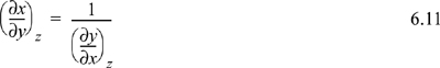
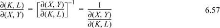
Basic Identities
Frequently as we manipulate derivatives we obtain derivatives of the following forms which should be recognized.

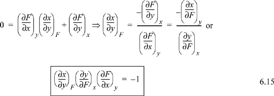
Triple Product Rule
Suppose F = F(x,y), then
Consider what happens when dF = 0 (i.e., at constant F). Then,
Two Other Useful Relations
First, for any partial derivative involving three variables, say x, y, and F, we can interpose a fourth variable z using the chain rule:
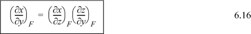
Another useful relation is found by a procedure known as the expansion rule. The details of this expansion are usually not covered in introductory calculus texts:
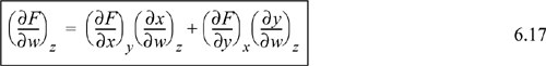
Recall that we started with a function F = F(x,y). If you look closely at the expansion rule, it provides a method to evaluate a partial derivative (∂F/∂w)z in terms of (∂x/∂w)z and (∂y/∂w)z. Thus, we have transformed the calculation of a partial derivative of F to partial derivatives of x and y. This relation is particularly useful in manipulation of the fundamental relations S, U, H, A, and G when one of these properties is substituted for F, and the natural variables are substituted for x and y. We will demonstrate this in Examples 6.1 and 6.2. Look again at Eqn. 6.17. It looks like we have taken the differential expression of Eqn. 6.14 and divided through the differential terms by dw and constrained to constant z, but this procedure violates the rules of differential operators. What we have actually done is not nearly this simple.2 However, looking at the equation this way provides a fast way to remember a complicated-looking expression.
Exact Differentials
In this section, we apply calculus to the fundamental properties. Our objective is to derive relations known as Maxwell’s relations. We begin by reminding you that we can express any state property in terms of any other two state properties. For a function which is only dependent on two variables, we can obtain the following differential relation, called in mathematics an exact differential.
Developing the ability to express any state variable in terms of any other two variables from the set {P, T, V, S} as we have just done is very important. But the equation looks a little formidable. However, the fundamental property relationship says:
Comparison of the above equations shows that:
This means that the derivatives in Eqn. 6.18 are really properties that are familiar to us. Likewise, we can learn something about formidable-looking derivatives from enthalpy:
But the result of the fundamental property relationship is:
dH = TdS + VdP
Comparison shows that:
T = (∂H/∂S)P and V = (∂H/∂P)S
Now, we see that a definite pattern is emerging, and we could extend the analysis to Helmholtz and Gibbs energy. We can, in fact, derive relations between certain second derivatives of these relations. Since the properties U, H, A, and G are state properties of only two other state variables, the differentials we have given in terms of two other state variables are known mathematically as exact differentials; we may apply properties of exact differentials to these properties. We show the features here; for details consult an introductory calculus textbook. Consider a general function of two variables: F = F(x,y), and
For an exact differential, differentiating with respect to x we can define some function M:
Similarly differentiating with respect to y:
Taking the second derivative and recalling from multivariable calculus that the order of differentiation should not matter,

This simple observation is sometimes called Euler’s reciprocity relation.3 To apply the reciprocity relation, recall the total differential of enthalpy considering H = H(S,P):
Considering second derivatives:
A similar derivation applied to each of the other thermodynamic functions yields the equations known as Maxwell’s relations.
Maxwell’s Relations
Example 6.1. Pressure dependence of H
Derive the relation for ![]() and evaluate the derivative for: a) water at 20°C where
and evaluate the derivative for: a) water at 20°C where ![]() and
and ![]() , ρ = 0.998 g/cm3; b) an ideal gas.
, ρ = 0.998 g/cm3; b) an ideal gas.
Solution
First, consider the general relation dH = TdS + VdP. Applying the expansion rule,

by a Maxwell relation, the entropy derivative may be replaced
which is valid for any fluid.
a. Plugging in values for liquid water,
Therefore, within 6% at room temperature, ![]() for liquid water as used in Eqn. 2.42 on page 59 and Example 2.6 on page 60.
for liquid water as used in Eqn. 2.42 on page 59 and Example 2.6 on page 60.
b. For an ideal gas, we need to evaluate (∂V/∂T)P. Applying the relation to V = RT/P, (∂V/∂T)P = R/P. Inserting into Eqn. 6.33, enthalpy is independent of pressure for an ideal gas.
A non-ideal gas will have a different partial derivative, and the enthalpy will depend on pressure as we will show in Chapter 8.
Example 6.2. Entropy change with respect to T at constant P
Evaluate (∂S/∂T)P in terms of CP, CV, T, P, V, and their derivatives.
Solution
CP is the temperature derivative of H at constant P. Let us start with the fundamental relation for enthalpy and then apply the expansion rule. Recall, dH = TdS + VdP.
Applying the expansion rule, Eqn. 6.17, we find,
Applying the basic identity of Eqn. 6.12 to the second term on the right-hand side, since P appears in the derivative and as a constraint the term is zero,
But the definition of the left-hand side is given by Eqn. 2.36: CP ≡ (∂H/∂T)P.
Therefore, (∂S/∂T)P = CP/T, which we have seen before as Eqn. 4.31, and we have found that the constant-pressure heat capacity is related to the constant-pressure derivative of entropy with respect to temperature. An analogous analysis of U at constant V results in a relation between the constant-volume heat capacity and the derivative of entropy with respect to temperature at constant V. That is, Eqn. 4.30,
(∂S/∂T)V = CV/T
Example 6.3. Entropy as a function of T and P
Derive a general relation for entropy changes of any fluid with respect to temperature and pressure in terms of CP, CV, P, V, T, and their derivatives.
Solution
First, since we choose T, P to be the controlled variables, applying Eqn. 6.14
but (∂S/∂T)P = CP/T as derived above, and Maxwell’s relations show that

This useful expression is ready for application, given an equation of state which describes V(T,P).
Note that expressions similar to Eqn. 6.37 can be derived for other thermodynamic variables in an analogous fashion. These represent powerful short-hand relations that can be used to solve many different process-related problems. In addition to Eqn. 6.37, some other useful expressions are listed below. These are so frequently useful that they are also tabulated on the front flap of the text for convenient reference.
The Importance of Derivative Manipulations
One may wonder, “What is so important about the variables CP, CV, P, V, T, and their derivatives?” The answer is that these properties are experimentally measureable. Engineers have developed equations of state written in terms of these fundamental properties. Briefly, an equation of state provides the link between P, V, and T. So, we can solve for all the derivatives by knowing an equation for P = P(V,T) and add up all the changes. Properties like H, U, and S are not considered measurable because we don’t have gauges that measure them. Look back at the descriptions in Section 6.2. CP and CV are considered measurable though they are typically measured using the energy balance with temperature changes. A goal of derivative manipulations is to convert derivatives involving unmeasurable properties into derivatives involving measurable properties.
As for CP and CV, we should actually be very careful about specifying when we are referring to the CP of a real fluid or the ![]() of an ideal gas, but the distinction is frequently not made clear in literature. You may need to recognize from the context of the source whether CP is for the ideal gas or something else. In most cases, the intent is to apply
of an ideal gas, but the distinction is frequently not made clear in literature. You may need to recognize from the context of the source whether CP is for the ideal gas or something else. In most cases, the intent is to apply ![]() at low density to account for temperature effects and then to apply a correction factor of dV or dP to account for non-ideal gas density or pressure effects. In this way, in Chapter 8 we compute ΔU, ΔH, ΔS, ΔA, or ΔG from any initial (or reference) condition to any final condition and we can imagine compiling the results in the format of the steam tables for any particular compound.
at low density to account for temperature effects and then to apply a correction factor of dV or dP to account for non-ideal gas density or pressure effects. In this way, in Chapter 8 we compute ΔU, ΔH, ΔS, ΔA, or ΔG from any initial (or reference) condition to any final condition and we can imagine compiling the results in the format of the steam tables for any particular compound.
Test Yourself
Sketch two subcritical isotherms and two supercritical isotherms. Using the isotherms, describe how the following derivatives could be obtained numerically: (∂P/∂T)V, (∂V/∂T)P, (∂P/∂V)T. Compare the relative sizes of the derivatives for liquids and gases.
Important Measurable Derivatives
Two measurable derivatives are commonly used to discuss fluid properties, the isothermal compressibility and the isobaric coefficient of thermal expansion. The isothermal compressibility is
The isobaric coefficient of thermal expansion is
A similar commonly used property is the Joule-Thomson coefficient defined by

It is easy to see how this property relates to the physical situation of temperature changes as pressure drops through an isenthalpic throttle valve, though it is not considered measurable because of the constraint on H. The manipulation in terms of measurable properties is considered in Problem 6.8.
The next two examples illustrate the manner in which derivative manipulations are applied with a particularly simple equation of state to obtain an expression for ΔS. In this chapter, we establish this conceptual approach and the significant role of an assumed equation of state. The next chapter focuses on the physical basis of developing a reasonable equation of state. Since the derivative manipulations are entirely rigorous, we come to understand that all the approximations in all thermodynamic modeling are buried in the assumptions of an equation of state. Whenever an engineering thermodynamic model exhibits inaccuracy, the assumptions of the equation of state must be reconsidered and refined in the context of the particular application.
Example 6.4. Entropy change for an ideal gas
A gas is being compressed from ambient conditions to a high pressure. Devise a model equation for computing ΔS(T,P). Assume the ideal gas equation of state.
Solution
We begin with the temperature effect at (constant) low pressure. By Eqn. 6.37,
Having accounted for the temperature effect at constant pressure, the next step is to account for the pressure effect at constant temperature. The derivative (∂V/∂T)P is required.
Putting it all together,
Assuming ![]() is independent of T and integrating,
is independent of T and integrating,
Once again, we arrive at Eqn. 4.29, but this time, it is easy to recognize the necessary changes for applications to non-ideal gases. That is, we must simply replace the P-V-T relation by a more realistic equation of state when we evaluate derivatives.
Example 6.5. Entropy change for a simple nonideal gas
A gas is compressed from ambient conditions to a high pressure. Devise a model equation for computing ΔS(T,P) with the equation of state: V = RT/P + (a + bT), where a and b are constants.
Solution
Substituting the new equation of state and following the previous example,
(∂V/∂T)P = R/P + b
We can still apply ![]() because we could be careful to calculate temperature effects at low P before calculating the pressure effect. Inserting into Eqn. 6.37,
because we could be careful to calculate temperature effects at low P before calculating the pressure effect. Inserting into Eqn. 6.37,
Assuming ![]() is independent of T and integrating,
is independent of T and integrating,
Equations of state can be much more complicated than this one, motivating us to carefully contemplate the most efficient manner to organize our derivative relations to transform complex equations of state into useful engineering models. The departure function formalism as described in Chapter 8 provides this kind of efficiency. A key manipulation in that chapter will be the volume dependence of properties at constant temperature.
Example 6.6. Accounting for T and V impacts on energy
Derive an expression for ![]() in terms of measurable properties. (a) Evaluate for the ideal gas. (b) Evaluate for the van der Waals equation of state, P = RT/(V – b) – a/V.
in terms of measurable properties. (a) Evaluate for the ideal gas. (b) Evaluate for the van der Waals equation of state, P = RT/(V – b) – a/V.
Solution
Beginning with the fundamental relation for dU,
dU = TdS – PdV
Applying the expansion rule
Using a Maxwell relation and a basic identity
a. For an ideal gas, P = RT/V
Thus, internal energy of an ideal gas does not depend on volume (or pressure) at a given T.
b. For the van der Waals equation,
Another important application of derivative manipulations is in deriving meaningful connections between U, H, A, G, and S. We illustrate this kind of application with two examples. The first is a fairly simple development of the relation between energy and Helmholtz energy; the relation arises frequently in applications in Unit III of the text. The second example pertains to the Einstein solid model that was used to demonstrate the connection between the microscopic and macroscopic definitions of entropy. This second example involves more tedious calculus, but reveals broad insights related to chemistry and spectroscopy as well as entropy and heat capacity.
Example 6.7. The relation between Helmholtz energy and internal energy
Express the following in terms of U, H, S, G, and their derivatives: (∂(A/RT)/∂T)V.
Solution
Applying the product rule,
Applying Eqn. 6.6 and the definition of A,
Rearranging, and introducing a common definition β ≡ 1/kT,
The significance of Eqn. 6.47 is that one can easily transform from Helmholtz energy to internal energy and vice versa by integrating or differentiating. This is especially easy when the temperature dependence is expressed as a polynomial.
We are now in a position to return to the discussion of the relation between entropy and temperature that was begun in Chapter 4. Many experimental observations circa 1900 were challenging the conventional theories of atomic motions. It seemed that particles the size of atoms, and smaller, might be moving in discrete steps of energy, instead of continuous energies, and this altered the behavior that was being observed. For example, the covalent bond of nitrogen appears to vibrate classically at high temperature, but to become rigid at low temperature. The nature of this transition and its impact on heat capacity require explanation. The Einstein solid model was a major milestone in resolving many of these peculiar observations.
Albert Einstein wrote 45 articles between 1901 and 1907. Of these, 11 were about thermodynamics, 24 were reviews about thermodynamics, 7 were about relativity, 1 was about electromagnetism, and 2 were about the photoelectric effect. Of course, his revolutionary works were about relativity and the photoelectric effect because they opened new vistas of physical insight. But his work on heat capacity might arguably have had the broader immediate impact. Einstein showed that a very simple quantized theory predicted the experimental observations that classical theory could not explain. The following example applies derivative manipulations to obtain heat capacity from the entropy and demonstrate that the heat capacity approaches zero at zero Kelvin.
Example 6.8. A quantum explanation of low T heat capacity
The result of the Einstein solid model, from Example 4.2 on page 141, can be rearranged to:
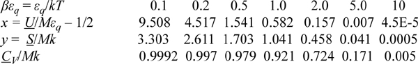
where y = S/Mk and x = <qM> = U/Mεq – 1/2. Use these results to derive the temperature dependence of S/Mk, U/Mεq – 1/2, and CV as instructed.
a. Derive a formula for CV/Mk. Tabulate values of y, x, and CV/Mk versus βεq at βεq = {0.1, 0.2, 0.5, 1, 2, 5, 10}. Recall that β = 1/kT.
b. The following data have been tabulated for silver by McQuarrie.a Iterate on εq/k to find the best fit and plot CV/Mk versus kT/εq, comparing theory to experiment. Also indicate the result of classical mechanics with a dashed line.
Solution
a. Noting that (∂S/∂T)V = CV/T, a logical step is to take (∂y/∂T)V = CV/MkT.
Note that the CV terms cancel, seeming to defeat the purpose, but substitute anyway and recognize internal energy is embedded.
We may not have obtained CV as expected, but we obtained U(T), so it is straightforward to evaluate CV from its definition: CV = (∂U/∂T)V.
Multiplying both sides by T for convenience,
Multiplying and dividing by k on the left-hand side,
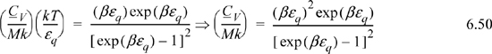
Varying βεq and tabulating energy and entropy, noting that the lowest temperatures are on the right, values of U and x = <qM> are calculated by Eqn. 6.49, S/Mk by 6.48, and CV/Mk by 6.50. We can see that the heat capacity goes to zero as 0 K is approached.
b. As discussed in Example 4.2 on page 141, each atom has three possible directions of motion, so M = 3N. Therefore, the quantum mechanical formula is CV/(Mk) = CV/(3Nk) = CV/(3R).
The classical value of the solid heat capacity can be deduced by considering the degrees of freedom.b Kinetic and potential energy each contribute a degree of freedom for a bond. Recalling from Section 2.10 that each degree of freedom contributes R/2 to CV, CVcs = 2(Nk/2)(M/N) = Mk = 3nR, or CVcs = 3R where CVcs is the heat capacity of the classical solid. Note that the table in part (a) approaches the classical result at high temperature, CVcs/3R = 1.
CV/Mk is fitted in Excel by naming a cell as εq/k and applying Eqn. 6.50. The function SUMXMY2 was used to compute Σ(calc – expt)2. Minimization with the Solver gives εq/k = 159 K. Values of CV/3R and CV/Mk at εq/k = 159 K are tabulated below.

a. McQuarrie, D.A., 1976. Statistical Mechanics. New York, NY: Harper & Row, p. 205.
b. The degrees of freedom for kinetic and potential energy discussed here are different from the degrees of freedom for the Gibbs phase rule. See also, Section 2.10.
Einstein’s expression approaches zero too quickly relative to the experimental data, but it explains the large qualitative difference between the classical theory and experiment. Several refinements have appeared over the years and these fit the data more closely, but the key point is that quantized energy leads to freezing out the vibrational degrees of freedom at temperatures substantially above 0 K. This phenomenology also applies to the vibrations of polyatomic molecules, as explored in the homework for a diatomic molecule. The weaker bond energy of bromine relative to nitrogen is also evident in its higher value of CP/R as listed on the back flap. From a broader perspective, Einstein’s profound insight was that quantized energy meant that thermal entropy could be conceived in a manner analogous to configurational entropy except by putting particles in energy levels rather than putting particles in boxes spatially. In this way, we can appreciate that the macroscopic and microscopic definitions of entropy are analogous applications of distributions.
Hints on Manipulating Partial Derivatives
1. Learn to recognize ![]() and
and ![]() as being related to CP and CV, respectively.
as being related to CP and CV, respectively.
2. If a derivative involves entropy, enthalpy, or Helmholtz or Gibbs energy being held constant, e.g., ![]() , bring it inside the parenthesis using the triple product relation (Eqn. 6.15). Then apply the expansion rule (Eqn. 6.17) to eliminate immeasurable quantities. The expansion rule is very useful when F of that equation is a fundamental property.
, bring it inside the parenthesis using the triple product relation (Eqn. 6.15). Then apply the expansion rule (Eqn. 6.17) to eliminate immeasurable quantities. The expansion rule is very useful when F of that equation is a fundamental property.
3. When a derivative involves {T, S, P, V} only, look to apply a Maxwell relation.
4. When nothing else seems to work, apply the Jacobian method.4 The Jacobian method will always result in derivatives with the desired independent variables.
Example 6.9. Volumetric dependence of CV for ideal gas
Determine how CV depends on volume (or pressure) by deriving an expression for (∂CV/∂V)T. Evaluate the expression for an ideal gas.
Solution
Following hint #1 and applying Eqn. 4.30:
By the chain rule:
Changing the order of differentiation:
For an ideal gas, P = RT/V, we have ![]() in Example 6.6:
in Example 6.6:
Thus, heat capacity of an ideal gas does not depend on volume (or pressure) at a fixed temperature. (We will reevaluate this derivative in Chapter 7 for a real fluid.)
Example 6.10. Application of the triple product relation
Evaluate (∂S/∂V)A in terms of CP, CV, T, P, and V. Your answer may include absolute values of S if it is not a derivative constraint or within a derivative term.
Solution
This problem illustrates a typical situation where the triple product rule is helpful because the Helmholtz energy is held constant (hint #2). It is easiest to express changes in the Helmholtz energies as changes in other variables. Applying the triple product rule:
(∂S/∂V)A = –(∂A/∂V)S/(∂A/∂S)V
Applying the expansion rule twice, dA = –PdV – SdT ⇒ (∂A/∂V)S = – P – S(∂T/∂V)S and (∂A/∂S)V = 0 – S(∂T/∂S)V. Recalling Eqn. 4.30 and converting to measurable derivatives:
Substituting:
Example 6.11. Master equation for an ideal gas
Derive a master equation for calculating changes in U for an ideal gas in terms of {V, T}.
Solution
Applying results of the previous examples:
Notice that this expression is more complicated than the fundamental property relation in terms of {S, V}. As we noted earlier, this is why {S, V} are the natural variables for dU, rather than {T,V} or any other combination. For an ideal gas, we can use the results of Example 6.6 to find:
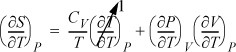
Example 6.12. Relating CP to CV
Derive a general formula to relate CP and CV.
Solution
Start with an expression that already contains one of the desired derivatives (e.g., CV) and introduce the variables necessary to create the second derivative (e.g., CP). Beginning with Eqn. 6.38,
and using the expansion rule with T at constant P,
 , where the left-hand side is
 ![]() .
.
Exercise:
Verify that the last term simplifies to R for an ideal gas.
Owing to all the interrelations between all the derivatives, there is usually more than one way to derive a useful result. This can be frustrating to the novice. Nevertheless, patience in attacking the problems, and attacking a problem from different angles, can help you to visualize the structure of the calculus in your mind. Each problem is like a puzzle that can be assembled in multiple ways. Patience in developing these tools is rewarded with a mastery of the relations that permit quick insight into the easiest way to solve problems.
6.3. Advanced Topics
Hints for Remembering the Auxiliary Relations
Auxiliary relations can be easily written by memorizing the fundamental relation for dU and the natural variables for the other properties. Note that {T,S} and {P,V} always appear in pairs, and each pair is a set of conjugate variables. A Legendre transformation performed on internal energy among conjugate variables changes the dependent variable and the sign of the term involving the conjugate variables. For example, to transform P and V, the product PV is added to U, resulting in Eqn. 6.5. To transform T and S, the product TS is subtracted: A = U – TS, dA = dU – TdS – SdT = –SdT – PdV. The pattern can be easily seen in the “Useful Derivatives” table on the front book end paper. Note that {T,S} always appear together, and {P,V} always appear together, and the sign changes upon transformation.
Jacobian Method of Derivative Manipulation
A partial derivative may be converted to derivatives of measurable properties with any two desired independent variables from the set {P,V,T}. Jacobian notation can be used to manipulate partial derivatives, and there are several useful rules for manipulating derivatives with the notation. The Joule-Thomson coefficient is a derivative that indicates how temperature changes upon pressure change at fixed enthalpy, ![]() , which is written in Jacobian notation as
, which is written in Jacobian notation as ![]() . Note how the constraint of constant enthalpy is incorporated into the notation. The rules for manipulation of the Jacobian notation are,
. Note how the constraint of constant enthalpy is incorporated into the notation. The rules for manipulation of the Jacobian notation are,
1. Jacobian notation represents a determinant of partial derivatives,
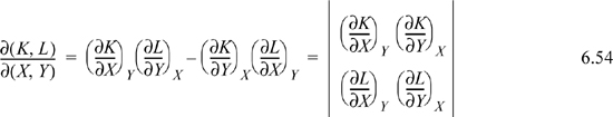
The Jacobian is particularly simple when the numerator and denominator have a common variable,
which is a special case of Eqn. 6.54.
2. When the order of variables in the numerator or denominator is switched, the sign of the Jacobian changes. Switching the order of variables in both the numerator and denominator results in no sign change due to cancellation. Consider switching the order of variables in the numerator,
3. The Jacobian may be inverted.
4. Additional variables may be interposed. When additional variables are interposed, it is usually convenient to invert one of the Jacobians.

Manipulation of Derivatives
Before manipulating derivatives, the desired independent variables are selected. The selected independent variables will be held constant outside the derivatives in the final formula. The general procedure is to interpose the desired independent variables, rearrange as much as possible to obtain Jacobians with common variables in the numerator and denominator, write the determinant for any Jacobians without common variables; then use Maxwell relations, the expansion rule, and so on, to simplify the answer.
1. If the starting derivative already contains both the desired independent variables, the result of Jacobian manipulation is redundant with the triple product rule. The steps are: 1) write the Jacobian; 2) interpose the independent variables; 3) rearrange to convert to partial derivatives.
Example: Convert ![]() to derivatives that use T and P as independent variables.
to derivatives that use T and P as independent variables.

and the numerator can be simplified using the expansion rule as presented in Example 6.1.
2. If the starting derivative has just one of the desired independent variables, the steps are: 1) write the Jacobian; 2) interpose the desired variables; 3) write the determinant for the Jacobian without a common variable; 4) rearrange to convert to partial derivatives.
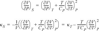
Example: Find a relation for the adiabatic compressibility, ![]() in terms of derivatives using T, P as independent variables.
in terms of derivatives using T, P as independent variables.
Now, including a Maxwell relation as we simplify the second term in square brackets, and then combining terms:
3. If the starting derivative has neither of the desired independent variables, the steps are: 1) write the Jacobian; 2) interpose the desired variables; 3) write the Jacobians as a quotient and write the determinants for both Jacobians; 4) rearrange to convert to partial derivatives.
Example: Find ![]() in measurable properties using P and T as independent variables.
in measurable properties using P and T as independent variables.

Writing the determinants for both Jacobians:
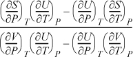
Now, using the expansion rule for the derivatives of U, and also introducing Maxwell relations,
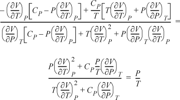
The result is particularly simple. We could have derived this directly if we had recognized that S and V are the natural variables for U. Therefore, dU = TdS – P dV = 0, ![]() . However, the exercise demonstrates the procedure and power of the Jacobian technique even though the result will usually not simplify to the extent of this example.
. However, the exercise demonstrates the procedure and power of the Jacobian technique even though the result will usually not simplify to the extent of this example.
6.4. Summary
We have seen in this chapter that calculus provides powerful tools permitting us to calculate changes in immeasurable properties in terms of other measurable properties. We started by defining additional convenience functions A, and G by performing Legendre transforms. We then reviewed basic calculus identities and extended throughout the remainder of the chapter. The ability to perform these manipulations lays the foundation for the development of general methods to calculate thermodynamic properties for any chemical from P-V-T relations. If we only had a general relation that perfectly described P=P(V,T) for all the chemicals in the universe, it could be combined with the tools in this chapter to compute any property required by the energy and entropy balances. At present, no such perfect equation exists. This means that we need to understand what makes it so difficult to develop such an equation and how the various available equations can be applied in various situations to achieve reasonable and continuously improving estimates.
Important Equations
The procedures developed in this chapter are what is important. They provide a basis for transforming one set of derivatives into another and for thinking systematically about how variables relate to one another. The basic identities 6.11–6.17 combine with the fundamental properties for the remainder of the chapter. Nevertheless, several equations stand out as a summary of the results that can be rearranged to a desired form relatively quickly. These are the Maxwell Eqns. 6.29–6.32, and also some intermediate manipulations 6.37–6.41. They are included on the front flap of the text-book for your convenience. Eqn. 6.47 stands out as an equation for long term reference because it relates the Helmholtz energy to the internal energy. That is a key step when we turn to consideration of solution models. Also, when combined with a similar relation is for compressibility factor in Chapter 7, the central role of Helmholtz energy in thermodynamic properties becomes apparent.
Test Yourself
1. What are the restrictions necessary to calculate one state property in terms of only two other state variables?
2. When integrating Eqn. 6.53, under what circumstances may CV be taken out of the integral?
3. May Eqn. 6.53 be applied to a condensed phase?
4. Is the heat capacity different for liquid acetone than for acetone vapor?
5. Can the tabulated heat capacities be used in Eqn. 6.53 for gases at high pressure?
6.5. Practice Problems
P6.1. Express in terms of P, V, T, CP, CV, and their derivatives. Your answer may include absolute values of S if it is not a derivative constraint or within a derivative.
a. (∂H/∂S)V
b. (∂H/∂P)V
c. (∂G/∂H)P
(ANS. (a) T[1+V/CV(∂P/∂T)v] (b) Cv(∂T/∂P)v+V (c) –S/CP)
6.6. Homework Problems
6.1. CO2 is given a lot of credit for global warming because it has vibrational frequencies in the infrared (IR) region that can absorb radiation reflected from the Earth and degrade it into thermal energy. The vibration at ε/k = 290K (903cm—1) is particularly important.
a. Plot Cvig/R versus T for CO2 in the range 200—400 K. Use the polynomial expression in the back of the book to estimate Cvig/R at 200 K as a reference. Also plot the polynomial expression on the same chart as a dashed line.
b. Use your Internet search skills to learn the wavelength range of the IR spectrum. How many wavelengths are there? What fraction does the wavelength at 903cm—1 comprise? If the Earth’s atmosphere was composed entirely of CO2, what fraction of IR energy could be absorbed by CO2?
c. The Earth’s atmosphere is really 380ppm CO2. If the absorption efficiency is proportional to the concentration, how much IR energy could be absorbed by CO2 in this case?
6.2. Express in terms of P, V, T, CP, CV, and their derivatives. Your answer may include absolute values of S if it is not a derivative constraint or within a derivative.
a. (∂G/∂P)T
b. (∂P/∂A)V
c. (∂T/∂P)S
d. (∂H/∂T)U
e. (∂T/∂H)S
f. (∂A/∂V)P
g. (∂T/∂P)H
h. (∂A/∂S)P
i. (∂S/∂P)G
6.3. Express the following in terms of U, H, S, A, and their derivatives.
a. Derive ![]() and
and ![]() in terms of measurable properties.
in terms of measurable properties.
b. dH = dU + d(PV) from the definition of H. Apply the expansion rule to show the difference between ![]() and
and ![]() is the same as the result from part (a).
is the same as the result from part (a).
6.5. In Chapter 2, internal energy of condensed phases was stated to be more weakly dependent on pressure than enthalpy. This problem evaluates that statement.
a. Derive ![]() and
and ![]() in terms of measurable properties.
in terms of measurable properties.
b. Evaluate ![]() and compare the magnitude of the terms contributing to
and compare the magnitude of the terms contributing to ![]() for the fluids listed in problem 5.6.
for the fluids listed in problem 5.6.
c. Evaluate ![]() for the fluids listed in problem 5.6 and compare with the values of
for the fluids listed in problem 5.6 and compare with the values of ![]() .
.
6.6. Express ![]() in terms of αP and/or κT.
in terms of αP and/or κT.
6.7. Express the adiabatic compressibility, ![]() , in terms of measurable properties.
, in terms of measurable properties.
6.8. Express the Joule-Thomson coefficient in terms of measurable properties for the following:
a. Van der Waals equation given in Example 6.6
b. An ideal gas.
a. Prove ![]() .
.
b. For an ideal gas along an adiabat, (P/Pi) = (T/Ti)Cp/R. Demonstrate that this equation is consistent with the expression from part (a).
6.10. Determine the difference CP – CV for the following liquids using the data provided near 20°C.
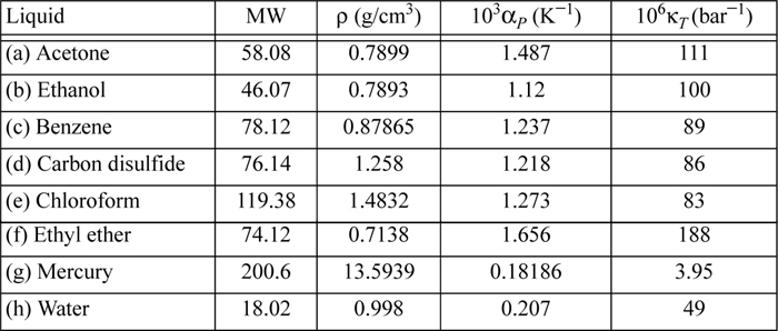
6.11. A rigid container is filled with liquid acetone at 20°C and 1 bar. Through heat transfer at constant volume, a pressure of 100 bar is generated. CP = 125 J/mol-K. (Other properties of acetone are given in problem 6.10.) Provide your best estimate of the following:
a. The temperature rise
b. ΔS, ΔU, and ΔH
c. The heat transferred per mole
6.12. The fundamental internal energy relation for a rubber band is dU = TdS – FdL where F is the system force, which is negative when the rubber band is in tension. The applied force is given by Fapplied = k(T)(L – L0) where k(T) is positive and increases with increasing temperature. The heat capacity at constant length is given by CL = α(L) + β(L)·T. Stability arguments show that α(L) and β(L) must provide for CL ≥ 0.
a. Show that temperature should increase when the rubber band is stretched adiabatically and reversibly.
b. Prof. Lira in his quest for scientific facts hung a weight on a rubber band and measured the length in the laboratory at room temperature. When he hung the rubber band with the same weight in the refrigerator, he noticed that the length of the rubber band had changed. Did the length increase or decrease?
c. The heat capacity at constant force is given by
Derive a relation for CF – CL and show whether this difference is positive, negative, or zero.
d. The same amount of heat flows into two rubber bands, but one is held at constant tension and the other at constant length. Which has the largest increase in temperature?
e. Show that the dependence of k(T) on temperature at constant length is related to the dependence of entropy on length at constant temperature. Offer a physical description for the signs of the derivatives.