
Chapter 14. Liquid-Liquid and Solid-Liquid Phase Equilibria
In the field of observation, chance favors the prepared mind.
Pasteur
The large magnitudes of the activity coefficients in the polymer mixing example should suggest an interesting possibility. Perhaps the escaping tendency for each of the polymers in the mixture is so high that they would prefer to escape the mixture to something besides the vapor phase. In other words, the components might separate into two distinct liquid phases. This can present quite a problem for blending plastics and recycling them because they do not stay blended. The next question is: How can we tell if a liquid mixture is stable as a single liquid phase? Also, crystallization is used for many pharmaceuticals and industrial products. An understanding of solid solubility is important for designing their separation.
Chapter Objectives: You Should Be Able to...
1. Compute LLE and VLLE phase behavior, including the ability to identify the onset of liquid instability.
2. Compute SLE phase behavior.
3. Predict the partitioning of a solute between two fluid phases (e.g., n-octanol and water).
4. Construct and interpret triangular phase diagrams.
14.1. The Onset of Liquid-Liquid Instability
Our common experience tells us that oil and water do not mix completely, even though both are liquids. If we consider equilibria between the two liquid phases, we can label one phase α and the other β. For such a system we can quickly show that the equilibrium compositions are given by
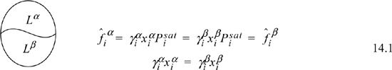
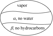
where superscripts identify the liquid phase. The coexisting compositions are known as mutual solubilities. Note that we have assumed an activity coefficient approach here even though we could formulate an entirely analogous treatment by an equation of state approach. There is also the possibility that three phases can coexist, two liquids and a vapor, which is illustrated below and is known as vapor-liquid-liquid equilibria, or VLLE. In this case we have an additional fugacity relation for the gas phase, where we assume in the figure that the ideal gas law is valid for the vapor phase. An example of how such a system could be solved is given below. The phase equilibria can be solved by starting with whichever two phases we know the most about, and filling in the details for the third phase.
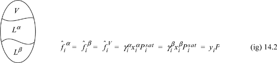
Example 14.1. Simple vapor-liquid-liquid equilibrium (VLLE) calculations
At 25°C, a binary system containing components 1 and 2 is in a state of three-phase LLVE. Analysis of the two equilibrium liquid phases (α and β) yields the following compositions:
![]()
Vapor pressures for the two pure components at 25°C are ![]() and
and ![]() .
.
Making reasonable assumptions, determine good estimates for the following.
a. The activity coefficients γ1 and γ2 (use Lewis-Randall standard states).
b. The equilibrium pressure.
c. The equilibrium vapor composition.
Solution
Assume ![]() because these are practically pure in the specified phases.
because these are practically pure in the specified phases.
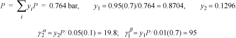
We also can determine activity coefficients from a theory to determine infinitely dilute concentrations. When a phase is nearly pure, the activity coefficient is nearly one at the same time xi is nearly one.
Example 14.2. LLE predictions using Flory-Huggins theory: Polymer mixing
One of the major problems with recycling polymeric products is that different polymers do not form miscible solutions with each other, but form highly nonideal solutions. To illustrate, suppose 1 g each of two different polymers (polymer A and polymer B) is heated to 127°C and mixed as a liquid. Estimate the mutual solubilities of A and B using the Flory-Huggins equation. Predict the energy of mixing using the Scatchard-Hildebrand theory. Polymer data:

Solution
This is the same mixture that we considered as an equal-weight-fraction mixture in Example 12.5. Based on that calculation, we know that the solution is highly nonideal. We must now iterate on the guessed solubilities until the implied activity coefficients are consistent. Let’s start by guessing that the two polymer phases are virtually pure and infinitely dilute in the other component.

Using Eqns. 11.46 and 11.47,
Since ![]() , then
, then ![]() and
and ![]() .
.
Good guess. The polymers are totally immiscible. No further iterations are needed.
14.2. Stability and Excess Gibbs Energy
Expressions for activity coefficients are the same for LLE as they are for VLE. The difference is that multiple liquid compositions can give the same activities or total pressure at a given temperature. This behavior is implied in Fig. 11.10, where we commented that the calculated lines indicate LLE. The time has come to analyze why this happens and how to properly represent the phase behavior of a system with two liquid phases.
Keep in mind that nature dictates phase stability by minimizing the Gibbs energy when T and P are fixed. Gibbs energies of mixtures using the one-parameter Margules equation for three values of A12 are plotted in Fig. 14.1 (the curves). In this plot, the important quantity is the Gibbs energy of the mixture G. In Fig. 14.1, the endpoints represent the values of Gi = Hi – TSi for the pure components, where the references states have been arbitrarily chosen, and only component 2 is at its reference state. If we imagine computing the Gibbs energy of two separate beakers containing the two separate components on the basis of one mole of total fluid, we see that this overall molar Gibbs energy is simply a molar average of the two component Gibbs energies along line 1 in the plot. There is no contribution from the entropy of mixing, because they are not mixing; they are in separate beakers. Substituting (1–x1) for x2 in this molar average formula shows that this formula is simply a linear relation in terms of x1. Deviations from this line are the changes due to the mixing process. Note how the shape of the Gibbs energy changes with the value of A12. Since ![]() , then rearranging,
, then rearranging,


Figure 14.1. Illustration of the Gibbs energy of a mixture represented by the Margules one-parameter equation.
where the last term represents the sum of component enthalpies represented by the upper straight line. The increasing excess Gibbs energy of mixing (larger A12) ultimately causes a “w-shaped” curve to form. The individual contributions of Eqn. 14.3 to the Gibbs energy are shown in Fig. 14.2.

Figure 14.2. Illustration of the contributions to the Gibbs energy of a binary mixture when A12 = 3 and the pure component Gibbs energies are as in Fig. 14.1.
The procedure of summing together Gibbs energies along a line also applies to any tie line. As shown in Fig. 14.1, A12 = 1 leads to a situation where connecting any two compositions by a straight line gives a value of G at the overall composition that is higher than the G along the curve. Line 2 on the plot shows this for a mixture with an overall composition z1 = 0.4 and assuming that two phases are formed x1α ≈ 0.17 (point a) and x1β ≈ 0.74 (point b). The overall Gibbs energy would be given by point c on the tie line, G/RT = –0.15. However, if the mixture stays as one phase, along the mixture line the Gibbs energy would be G/RT = –0.23 (point c’), a lower value, which means this is more stable. (Note that c’ must be at the overall composition along the line, z1 = 0.4.) Since the curve for A12 = 1 is concave up, a straight line between two points always gives a higher value for two phases.
This situation is quite different when we consider the case where A12 = 3. Along this curve, the mixture at z1 = 0.5 would have G ≈ 0.31, (point d), if it remained as a single phase. However, if the solution splits into two phases, line 3 can be drawn between the compositions of the phases (one point on either side of d) as shown by points e ![]() and
and ![]() , and the overall energy is given by the intersection of this line with the overall composition z1 = 0.5 as shown by point d’. The lowest energy is obtained when the line is tangent to the humps as shown in the figure, where G/RT ≈ 0.18, (point d’). Then, by splitting into two phases, the system clearly has a lower value for G/RT. Any other line that is drawn would force point d’ to have a higher Gibbs energy than this point. (Try it.) Considering these points at different values of A12 indicates that there is no phase split unless there is a hump in G/RT that makes it concave down. Note that A12 must be positive to create this curvature. This means that the activity coefficients must be greater than one, and the system must also have positive deviations from Raoult’s law for VLE.
, and the overall energy is given by the intersection of this line with the overall composition z1 = 0.5 as shown by point d’. The lowest energy is obtained when the line is tangent to the humps as shown in the figure, where G/RT ≈ 0.18, (point d’). Then, by splitting into two phases, the system clearly has a lower value for G/RT. Any other line that is drawn would force point d’ to have a higher Gibbs energy than this point. (Try it.) Considering these points at different values of A12 indicates that there is no phase split unless there is a hump in G/RT that makes it concave down. Note that A12 must be positive to create this curvature. This means that the activity coefficients must be greater than one, and the system must also have positive deviations from Raoult’s law for VLE.
One more point needs to be made before working some examples. Note that the line construction seems similar to what was done for VLE in a flash calculation at the beginning of Chapter 10. In fact, this is completely analogous mathematically to the flash in those diagrams, and the lever rule applies. The ratios of the phases can be found in a similar fashion. The only difference is that two liquid phases are formed upon a liquid-liquid flash rather than a vapor and liquid flash. For the example in the figure above, the fraction of the overall mixture that is the α phase (left side of diagram) is given by ![]() , so the mixture of this example splits into equal portions of the two phases. Note that the compositions for points e and f are the same for any overall composition between the two points. So a different overall composition in a binary mixture shifts the relative amounts of the two phases, but not their composition. (This simplification does not hold for more components; the Gibbs phase rule says F = C – P + 2.)
, so the mixture of this example splits into equal portions of the two phases. Note that the compositions for points e and f are the same for any overall composition between the two points. So a different overall composition in a binary mixture shifts the relative amounts of the two phases, but not their composition. (This simplification does not hold for more components; the Gibbs phase rule says F = C – P + 2.)
14.3. Binary LLE by Graphing the Gibbs Energy of Mixing
Fig. 14.2 shows the contributions to the Gibbs energy of a mixture for A12 = 3 of Fig 14.1. The pure component Gibbs energies do not contribute to the curvature in the Gibbs energy of a mixture, and therefore are not needed for LLE calculations—we need just ΔGmix. In principle, all that is required to make predictions of LLE partitioning is some method of calculating activity coefficients. In this section we use specific models (MAB and UNIFAC) to demonstrate calculation of LLE using ΔGmix. The plotting/tangent line method can be extended to any activity coefficient model. This method is often the easiest method to use for binary solutions, though we show that it is subject to uncertainties from drawing/reading the tangent line.
The MAB and UNIFAC models are convenient for demonstrating the calculations, but there is a certain danger in applying too much confidence in such predictions. LLE is more sensitive to the accuracy of the activity coefficients than VLE. Furthermore, the empirical nature of UNIFAC means that the same parameter set, {amn}, is not generally accurate for both VLE and LLE, so a different predictive parameter set is used. As for the sensitivity problem, the best advice is not to take any predictions too seriously. They can be used as a guide to assess miscibility in a way that is slightly better than looking at solubility parameter tables, but should never be considered as a substitute for experimental data. With these cautions in mind, it is useful to show how LLE can be predicted using UNIFAC and MAB. We have provided the LLE parameters on the spreadsheet UNIFAC(LLE) within Actcoeff.xlsx, and within Matlab/gammaModels/unifacLLE.
Example 14.3. LLE predictions by graphing
Arce et al.a give the compositions for the tie lines in the system water(1) + propanoic acid(2) + methylethylketone (MEK)(3) at 298 K and 1 bar. As limiting conditions, the mutual solubilities of water + MEK (1CH3 + 1CH3CO + 1CH2) binary are also listed as x1α = 0.342, x1β = 0.922.
a. Use MAB to roughly estimate the water + MEK binary mutual solubilities to ± 5 mole%.
b. Use UNIFAC to roughly estimate the water + MEK binary mutual solubilities to ± 5 mole%.
Solution
a. A12 = (50.13 – 0)(15.06 – 9.70)(90.1 + 18.0)/(4·8.314·298) = 2.931, virtually the same as the parameter used above.
Adding GE/RT = A12x1x2 and ![]() gives ΔGmix/(RT). Using the drawing tool shows
gives ΔGmix/(RT). Using the drawing tool shows ![]() and
and ![]()
b. Selecting the appropriate groups from the UNIFAC menu, then copying the values of the activity coefficient, we can develop Figs. 14.3 and 14.4 using increments of xw = 0.05. In MATLAB we can set up a vector x1 = 0:0.05:1, and then insert a loop into unifacCallerLLE.m. Noting ![]() and programming the formula for ΔGmix/(RT).
and programming the formula for ΔGmix/(RT).

Figure 14.3. Gibbs energy of mixing in the water + MEK system as predicted by (a) MAB and (b) UNIFAC.

Figure 14.4. Activities of water and MEK as a function of mole fraction water as predicted by UNIFAC. The activity versus mole fraction plots will have a maximum when LLE exists. The dashed lines show the compositions where the activities of components are equal in both phases simultaneously.
Using the line drawing tool we obtain tangents at ![]() and
and ![]() .
.
These are sufficiently precise for the problem statement as given above. Note how the MAB model results in symmetric estimates of the compositions, a serious deficiency for LLE, and UNIFAC happens to be fairly close.
a. 1995. J. Chem. Eng. Data 40:225.
14.4. LLE Using Activities
Usually we require higher precision than obtained by graphing the Gibbs energy. Furthermore, we may encounter multicomponent mixtures, for which the extension of the above method is not straightforward. We can develop an entirely general method for computing the phase partitioning given relative activities in Eqn 14.1. In Fig. 14.4 are plotted the activities for the water + MEK system of Example 14.3. The extrema in the activity plot are characteristic of LLE. The vertical lines indicate the compositions where the activities are equal in each phase. The horizontal lines indicate the activity values. This analysis is a graphical solution to Eqn. 14.1. We need a method to search for this condition numerically. Rearranging Eqn. 14.1 we have,

Note that the K-ratios calculated using the ratio of mole fractions should be identical to the value calculated using the ratio of activity coefficients at the stable LLE condition. This form is entirely analogous to the K-ratios in VLE. To find this condition, we can use an LLE flash calculation. We can iterate on the system by assuming values for mole fractions, generating activity coefficients at those x values to get K-ratios and then generating new values for mole fractions from the K-ratios. If the loop is constructed properly, it will create a successive substitution algorithm that will converge.
We can develop such a procedure by noting for a binary mixture that ![]() must sum to unity. We can calculate the concentrations using the compositions
must sum to unity. We can calculate the concentrations using the compositions ![]() in the other phase, and use the K-ratio to generate a new guess of composition. The principle balance equation is
in the other phase, and use the K-ratio to generate a new guess of composition. The principle balance equation is ![]() which leads to
which leads to
The method is initialized by assuming the two phases are virtually immiscible with an infinitely dilute trace of the other component. The method is as follows.
1. Assume that phase β is nearly pure 1, ![]() , and α is nearly pure 2,
, and α is nearly pure 2, ![]() . These represent initialization of the iteration procedure. The procedure is most stable with an initial guess of mutual solubility outside the two-phase region.
. These represent initialization of the iteration procedure. The procedure is most stable with an initial guess of mutual solubility outside the two-phase region.
2. Calculate ![]() where the γi′s are evaluated at the initial compositions.
where the γi′s are evaluated at the initial compositions.
3. Calculate ![]() .
.
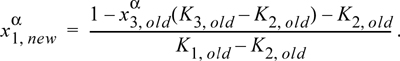
4. Calculate ![]() .
.
5. Determine γi,new values for each liquid phase from the xi,new values.
7. Replace all xi,old and Ki,old values with the corresponding new values.
8. Loop to step 3 until calculations converge. The calculations converge slowly.
A similar method for ternary systems is explored in a homework problem. Note that the Rachford-Rice flash method given for VLE in Section 10.3 can be adapted and provides an even more robust solution, but it is not as easy to implement in Excel without a macro. The method is provided in Matlab/Chap14/LLEflash.m.
Let us apply the binary algorithm above to the water and MEK system studied in the previous example.
Example 14.4. The binary LLE algorithm using MAB and SSCED models
Compute the mutual solubilities of water and MEK at 298 K and compare to the experimental data of Example 14.3 assuming the following models: (a) MAB (b) SSCED.
Solution
a. From Example 14.3, A12 = 2.931. The symmetry of the MAB model gives x1α = x2β = 1/exp(2.931) = 0.05335. Computing γi′s at these compositions, KW = 1.0084/13.83 = 0.0729; KMEK = 13.83/1.0084 = 13.72. Then Eqn. 14.5 gives ![]() ;
; ![]() for the first iteration. Unfortunately, the LLE calculations converge more slowly than VLE flash calculations. The calculations may drift a couple mole percent in compositions after they are changing at step sizes in the tenths of mole percents, so patience is required in converging the calculations. Section 14.9 provides details on setting up a macro or circular calculation. The table below summarizes the initial iterations. This same model is used above and the results are the same, but numerically known to better precision than the graphical method.
for the first iteration. Unfortunately, the LLE calculations converge more slowly than VLE flash calculations. The calculations may drift a couple mole percent in compositions after they are changing at step sizes in the tenths of mole percents, so patience is required in converging the calculations. Section 14.9 provides details on setting up a macro or circular calculation. The table below summarizes the initial iterations. This same model is used above and the results are the same, but numerically known to better precision than the graphical method.

b. The SSCED model gives:
k12 = (50.13 – 0)(15.06 – 9.70)/(4·27.94·18.88) = 0.1274.
From lnγ1∞ = 18[(27.94-18.88)2+2(0.1274)27.94(18.88)]/(8.314·298) = 1.573, x1α = 1/exp(1.573)= 0.2072.
Applying the same formulas to MEK: ![]() .
.
The table below shows the improved predictions from SSCED relative to MAB. Note how the molecular size difference is reflected by the much greater activity of trying to squeeze the large molecule among the small ones. This reflects a significantly improved insight for SSCED relative to the MAB model.
Iterating further on x1α through Eqn. 14.5 gives x1α = 0.2509.

A similar approach to this example could be applied to solve for the ternary problem of partitioning of the propanoic acid between water and MEK, starting with the above result and infinite dilution of the propanoic acid. By steadily increasing the propanoic acid and performing flash calculations each time, the impact of the propanoic acid on the water + MEK partitioning could be studied. Can you guess whether the propanoic acid causes relatively more MEK to dissolve into the water phase or vice versa? The answer is explored later in a homework problem.
14.5. VLLE with Immiscible Components
A special case of VLLE is obtained when one of the liquid-phase components is almost entirely insoluble in other components, and all other components are essentially insoluble in it, as occurs with many hydrocarbons with water. When a mixture forms two liquid phases, the mole fractions sum to unity in each of the phases. When a vapor phase coexists, it is a mixture of all components. The bubble pressure can be calculated using Eqn. 14.2, where the liquid phase fugacities are used to calculate the vapor phase partial pressures. For example, water and n-pentane are extremely immiscible. Applying the strategy used in Example 14.1, each liquid phase is essentially pure, resulting in the bubble pressure ![]() which is greater than the bubble point of either component. Rather than considering the bubble pressure, think about the bubble temperature. Since each component contributes to the partial pressure, the bubble temperature of a mixture of two immiscible liquids is lower than the bubble temperature of either pure component at a specified pressure. This phenomenon can be use to permit boiling at a lower temperature as shown in the next example.
which is greater than the bubble point of either component. Rather than considering the bubble pressure, think about the bubble temperature. Since each component contributes to the partial pressure, the bubble temperature of a mixture of two immiscible liquids is lower than the bubble temperature of either pure component at a specified pressure. This phenomenon can be use to permit boiling at a lower temperature as shown in the next example.
Example 14.5. Steam distillation
Consider a steam distillation with the vapor leaving the top of the fractionating column and entering the condenser at 0.1 MPa with the following analysis:
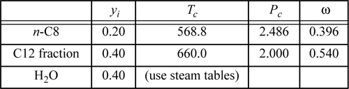
Assuming no pressure drop in the condenser and that the water and hydrocarbons are completely immiscible, calculate the maximum temperature which ensures complete condensation at 0.1 MPa. Use the shortcut K-ratio method for the hydrocarbons.
Solution
Apply the following notation to designate the phases:
The temperature that we seek is a bubble temperature of the liquid phases. The hydrocarbons and the water are essentially immiscible. We may approximate the hydrocarbon liquid phase, α, as an ideal solution of C8 and C12 with no water present. Therefore, two liquid phases will form: one of pure H2O and the other a mixture of 1/3 n-C8 + 2/3 C12 fraction. We may apply Raoult’s law with xw = 1 for water in the β phase. The vapor mixture is a single phase, however, and must conform to: ![]() .
.

So the bubble temperature with water present is ~95°C. Note that the bubble temperature is below the bubble temperature of pure water. What would it be without water?

Then, interpolating T ≈ 400 + (1 – 0.41)/(1.121 – 0.41)·40 = 433 K. Thus, we reduced the bubble temperature by 65°C in the steam distillation.
14.6. Binary Phase Diagrams
Liquid-liquid mutual solubilities in partially miscible systems change with temperature at a given pressure. Whether the solubilities increase or decrease can be due to a number of factors including hydrogen bonding. When one species H-bonds and the other does not, then as the temperature is raised and hydrogen bonds are broken, the fluids become more “similar,” and the LLE region decreases in size. The fluids can become miscible before the boiling point as shown in Fig. 19.12 on page 804 for methanol + cyclohexane. The liquid-liquid envelope is the dome in the figure. The temperature where the liquids become totally miscible is known as the upper critical solution temperature (UCST). Pressure affects the VLE curve, but has virtually no effect on the liquid phases or LLE. Thus, as the pressure is lowered, the VLE shifts to lower temperatures, and the VLE curve will overlap the LLE curve, giving a diagram similar to Fig. 16.2B on page 616, insets (e) and (f). For other systems that differ more greatly in vapor pressure, an azeotrope may not appear in the VLE and the diagram will appear as in Fig. 16.2A on page 616, insets (b) and (c).
When VLE is predicted by process simulators, the common default settings check for only one liquid phase. The result can be the odd diagrams as in Fig. 11.10 on page 435. How do we resolve such diagrams? Consider the T-x-y diagram in Fig. 14.5(a) for ethyl acetate + water generated using UNIQUAC parameters in the ASPEN Plus database. By default, ASPEN Plus models VLE; the dotted line is vapor and the dashed line is liquid. The solid line and dots have been added manually. Note the Lβ is in equilibrium with the left V branch all the way from 373 K to the two left-most dots. Likewise the Lα is in equilibrium with the right V branch all the way from the pure ethyl acetate boiling point to the two rightmost dots. The horizontal line is the VLLE condition because both L branches are simultaneously in equilibrium with the center V dot, and thus they are also in equilibrium with each other. The liquid compositions are at the outside dots and the vapor composition in this case is given by the center dot. This state is known as a heteroazeotrope because two liquid phases co-exist at the azeotrope condition. The odd loops below this VLLE temperature are not equilibrium states and are discarded. Fig. 14.5(b) is a comparison of experimental data with the diagram generated by specifying that the process simulator check for VLLE, though the dotted LLE lines are added manually to show the general type of expected behavior. Note how the lower loops are eliminated. The horizontal line method is easy to apply manually to any diagrams that you may generate.

Figure 14.5. (a) VLE predictions of ethyl acetate + water as predicted by literature parameters in ASPEN using UNIQUAC. The horizontal line and the dots have been added manually. (b) The correct phase behavior after specifying to check for VLLE. Note that the liquid-liquid envelope is sketched by hand based on general behavior that may be expected, not predicted, but the two liquid compositions at the bubble temperature are at the ends of the horizontal VLLE line. Data from Ellis, S. R. M.; Garbett, R. D. 1960. Ind. Eng. Chem. 52:385-388; Reichl, A.; et al, 1998. Fluid Phase Equil. 153:113–134; Lee, L.-S.; et al. 1996. J. Chem. Eng. Japan 96:427–438.
14.7. Plotting Ternary LLE Data
Graphical representation of ternary LLE data is important for design of separation processes. For ternary systems, triangular coordinates simultaneously represent all three mole fractions, or alternatively, all three weight fractions. Triangular coordinates are shown in Fig. 14.6(a), with a few grid lines displayed. The fraction of component A is represented by lines parallel to the BC axis: Along ![]() , the composition is xA = 0.25; along
, the composition is xA = 0.25; along ![]() , the composition is xA = 0.5. The fraction of B is represented by lines parallel to the AC axis; along
, the composition is xA = 0.5. The fraction of B is represented by lines parallel to the AC axis; along ![]() , the composition is xB = 0.5; along
, the composition is xB = 0.5; along ![]() , the composition is xB = 0.25. The fraction of C is along lines parallel to the AB axis; along
, the composition is xB = 0.25. The fraction of C is along lines parallel to the AB axis; along ![]() , xC = 0.5. Combining these conventions, at point h, xA = 0.25, xB = 0.25, xC = 0.5. An example of plotted LLE phase behavior is shown on triangular coordinates in Fig. 14.6(b). The compositions of coexisting α and β phases are plotted and connected with tie lines. The lever rule can be applied. For example, in Fig. 14.6(b), a feed of overall composition d will split into two phases: (moles β)/(moles α) =
, xC = 0.5. Combining these conventions, at point h, xA = 0.25, xB = 0.25, xC = 0.5. An example of plotted LLE phase behavior is shown on triangular coordinates in Fig. 14.6(b). The compositions of coexisting α and β phases are plotted and connected with tie lines. The lever rule can be applied. For example, in Fig. 14.6(b), a feed of overall composition d will split into two phases: (moles β)/(moles α) = ![]() , and (moles β)/(moles feed) =
, and (moles β)/(moles feed) = ![]() .
.
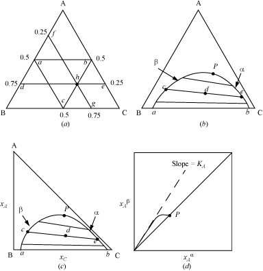
Figure 14.6. Illustrations of graphical representation of ternary data on triangular diagrams. (a) Illustration of grid lines on an equilateral triangle; (b) illustration of LLE on an equilateral triangle; (c) illustration of LLE on a right triangle; (d) illustration of tie-line data on a right triangle.
To specify the composition of an arbitrary phase α in a ternary system, only two mole fractions are required. Since the mole fractions must sum to unity, if ![]() and
and ![]() are known, then the third mole fraction can be found,
are known, then the third mole fraction can be found, ![]() . The subscripts may be interchanged, and the same constraints hold for phase β. Therefore, cartesian coordinates can be used to plot two mole (or weight) fractions of each phase. Fig. 14.6(c) presents the data from Fig. 14.6(b) on cartesian coordinates. The tie line and lever rule concepts also apply on this diagram. Tie line data can be plotted on cartesian coordinates as in Fig. 14.6(d). This representation of tie line data permits improved accuracy when interpolating between experimental tie lines. The slope of the tie line data, as presented in Fig. 14.6(d), is frequently linear near the origin; the slope of the line in this region is
. The subscripts may be interchanged, and the same constraints hold for phase β. Therefore, cartesian coordinates can be used to plot two mole (or weight) fractions of each phase. Fig. 14.6(c) presents the data from Fig. 14.6(b) on cartesian coordinates. The tie line and lever rule concepts also apply on this diagram. Tie line data can be plotted on cartesian coordinates as in Fig. 14.6(d). This representation of tie line data permits improved accuracy when interpolating between experimental tie lines. The slope of the tie line data, as presented in Fig. 14.6(d), is frequently linear near the origin; the slope of the line in this region is ![]() , which is the distribution coefficient, Ki. For the LLE phase behavior shown in Fig. 14.6, the B + C miscibility is increased by the addition of A. Along the phase boundary, the tie lines become shorter upon approach to point P, the Plait point. Note that at the Plait point, all distribution coefficients are one.
, which is the distribution coefficient, Ki. For the LLE phase behavior shown in Fig. 14.6, the B + C miscibility is increased by the addition of A. Along the phase boundary, the tie lines become shorter upon approach to point P, the Plait point. Note that at the Plait point, all distribution coefficients are one.
Other Examples of LLE Behavior
The ternary LLE of Fig. 14.6 is one of several common types. In this example, A + C is totally miscible (there is no immiscibility on the AC axis), as is A + B. When two of the three pairs of components are immiscible, the type of Fig. 14.7(a) can result, and when all three pairs have immiscibility regions, then type of Fig. 14.7(b) can result. In Fig. 14.7(b), the center region is LLL; since the T and P are fixed, any overall composition in the center triangle will split into the three phases of compositions a, b, and c, because F = C – P + 2 = 3 – 3 + 2 = 2.
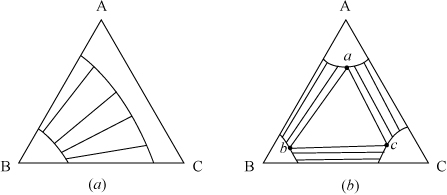
Figure 14.7. Illustration of other types of LLE behavior.
14.8. Critical Points in Binary Liquid Mixtures
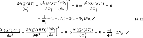
Referring back to Fig. 14.1, we may wish to find the combination of x1 and A12 where the system just begins to phase-split. This is known as a liquid-liquid critical point. If it is the highest T where two phases exist (called the UCST, upper critical solution temperature), then we must seek x1 where the concavity is equal to zero at only one composition (if it was less than zero anywhere, then we would just have a regular phase split, not a critical point—refer back to the curve for A12 = 3 in Fig. 14.1). If the concavity is equal to zero at x1 and greater everywhere else, then this must represent a minimum in the concavity as well a point where it equals zero. These two conditions provide two equations for the two unknowns, x1 and T, involved in determining the critical point. Recalling that concavity is given by the second derivative:
A generalization of these concepts to multicomponent mixtures gives
By analogy to the phase diagram for pure fluids, the locus where the second derivative equals zero represents the boundary of instability and is called the liquid-liquid spinodal.
Example 14.6. Liquid-liquid critical point of the Margules one-parameter model
Based on Fig. 14.1 and the discussion of concavity above, it looks like the value of A12 = 2 may be close to the critical point. Use Eqns. 14.6 and 14.7 to determine the exact value of the critical parameter.
Solution
Multiplying through by n and recognizing that we have previously performed the initial part of this derivation (see Eqns. 11.29–11.31) gives

Since this is a binary solution, there is a simple finite relationship between the derivative with respect to mole number and the derivative with respect to mole fraction, leading expeditiously to the expected conclusion:

From this example, we can draw a useful conclusion regarding the magnitude of activity coefficients that leads to immiscibility. Based on the Margules model, LLE should occur whenever A12 > 2, and a useful engineering rule of thumb for immiscibility is when the activity coefficients exceed the value of 7.4,

With the capability to determine immiscibility, it is possible to convey some background on one of the most significant scientific challenges currently occupying modern thermodynamicists. This is the problem of phase separation in polymer solutions and polymer blends. The same forces driving these phase separations lead to the extremely important problem of the collapse transition of a single polymer chain in a solvent or mixture. A special kind of collapse describes the protein folding problem. Imagine a bowl of spaghetti formed from a single noodle. After stretching the noodle until it is completely straight, release and watch it collapse into the bowl again. If the noodle was really a protein, it would collapse into exactly the same hooks and crooks as it was before being stretched. The folding is driven by hydrophobic effects, hydrogen bonding, and intramolecular interactions like helix formation. A complete understanding of this phenomenon would greatly facilitate drug design.
Limiting this introductory presentation to liquid-liquid equilibria, the phase partitioning of polymer mixtures is somewhat simpler in that we care only about collections of chains rather than the details of individual chains. Polymer solutions are classified differently from polymer blends in a manner that is superfluous to our mathematical analysis: polymer solutions are blends where the degree of polymerization of one of the components is unity (the small one is known as the solvent). With this minimal background, we can phrase the following problem:
Example 14.7. Liquid-liquid critical point of the Flory-Huggins model
Determine the critical value of the Flory-Huggins χ parameter considering the degrees of polymerization of each component.
Solution
Note that we have already solved this problem for the special case where the two components are identical in size. Then the excess entropy is zero, the volume fractions are equal to the mole fractions, and the Margules one-parameter model is recovered with A12 having nearly the same meaning as the Flory-Huggins χ parameter. To consider the problem of including the degree of polymerization, Nd, we must define the parameter with respect to a standard unit of volume. Nd is the number of monomer repeat units in the polymer. In the presentation below (and most other presentations of the same material), the volume of a monomer of component 1 is assigned as this standard volume (χ′ = Vstd·[δ1– δ2]2/RT; Vstd = V1/Nd,1). Note that we are introducing temperature dependence into χ′. Recalling the formula for the activity coefficient with this notational adaptation, the starting point (Eqn. 11.46) for this derivation becomes:

The next step is greatly simplified if we recognize a simple relationship that is very similar to the formula for computing the number average molecular weight from the weight fractions of each component. The analogous formula for the volume can be rearranged in terms of the volume ratio r = V2/V1 as follows:

Since this is a binary solution, there is a simple finite relationship between the derivative with respect to mole number and the derivative with respect to volume fraction, leading expeditiously to the general conclusion (note dΦ1 = –dΦ2):
which leads to two important results:

These results suggest that critical concentration decreases to zero with increasing polymer size but the critical temperature approaches a finite limit that is related to the solvent size.
There are a number of significant conclusions that may be drawn from the above example. First, for polymer solutions where (1) is the solvent (i.e., V1<<V2), the critical composition of polymer (2) approaches zero, and the critical temperature is a finite value that depends on the solvent and polymer molar volumes and solubility parameters. Furthermore, the critical temperatures for all polymers in a given solvent should be given by a universal curve with respect to molecular weight when reduced by the solubility parameter difference, although these predictions are only semi-quantitative due to the approximate nature of the Scatchard-Hildebrand theory. For blends where V1~V2, the critical temperature should be proportional to the molecular weight. We have applied several approximations in deriving these formulas, however. Therefore, significant efforts are currently underway to determine whether the formulas presented above are sufficiently accurate to describe the complex phase behavior often observed in polymer solutions and blends. Hanging in the balance is the ability to tailor-make polymer solutions and blends with many commercial advantages, because the ability to manipulate phase behavior successfully often relies on operating within the very sensitive critical region and knowing how to maneuver appropriately.
14.9. Numerical Procedures for Binary, Ternary LLE
Numerical procedures using Excel and MATLAB are provided in online supplements. The Excel procedure extends Actcoeff.xlsx and explains details on setting up the macro or circular reference for binary or ternary mixtures. The MATLAB Rachford-Rice procedure can be extended more easily to multicomponent mixtures.
14.10. Solid-Liquid Equilibria
Solid-liquid equilibria (SLE) calculations begin just as VLE and LLE calculations, by equating fugacities. From Eqn. 11.13, ![]() . The next step is to equate
. The next step is to equate ![]() and derive an equation to solve for temperature or composition depending on the problem statement. We have deliberately avoided substituting
and derive an equation to solve for temperature or composition depending on the problem statement. We have deliberately avoided substituting ![]() , however, as we did for VLE and LLE. This is because pure components below their melting temperature do not exist as liquids, so the vapor pressure is not relevant. This peculiarity necessitates a derivation to characterize a hypothetical liquid state. The treatment of the solid phase is usually much simpler, however, because most solids exist in a practically pure state. The purity of crystallized solid phases is one of the reasons for the prevalence of crystallization and filtration in the pharmaceutical industry.
, however, as we did for VLE and LLE. This is because pure components below their melting temperature do not exist as liquids, so the vapor pressure is not relevant. This peculiarity necessitates a derivation to characterize a hypothetical liquid state. The treatment of the solid phase is usually much simpler, however, because most solids exist in a practically pure state. The purity of crystallized solid phases is one of the reasons for the prevalence of crystallization and filtration in the pharmaceutical industry.
Pressure Effects
For SLE, as for LLE, pressure changes usually have very small effects on the equilibria unless the pressure changes are large (10 to 100 MPa), because the enthalpies and entropies of condensed phases are only weakly pressure-dependent. Since dG = RT d ln f = dH – T dS = V dP for a pressure change at constant T, the Gibbs energy and fugacity exhibit only small changes with pressure when the enthalpy and entropy exhibit small changes. (Recall that the Poynting correction factor is usually very near one.) In a mixture of liquids, the analysis must be done with partial molar enthalpies and partial molar entropies; however, these properties also depend only weakly on pressure. In the following subsections, we calculate properties at the triple-point, or other low pressures, and use the results at atmospheric pressure without pressure correction due to the weak pressure dependence.
SLE in a Single Component System
To begin our discussion, we will consider a single component. At 1 bar, water freezes at 0°C. Ice exists below this temperature and liquid exists above. From the principles of thermodynamics, the Gibbs energy is minimized at constant pressure and temperature; therefore, above 0°C, the Gibbs energy of liquid water must be lower than the Gibbs energy of solid water. In order to express this concept quantitatively, we must consider how the Gibbs energies of each of these phases changes with temperature.
The effect of temperature on the Gibbs energy of any phase may be determined most easily at constant pressure. We may write dG =–S dT + V dP, and recognize using the concepts of Chapter 6
(∂G/∂T)P = –S
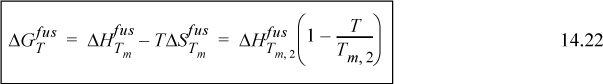
The temperature dependence of Gibbs energy is then dependent on the entropy of the phase. Entropy is a positive quantity; therefore, the Gibbs energy of any phase must decrease with increasing temperature. However, the entropy of a liquid phase is greater than the entropy of a solid phase; thus, the Gibbs energy of a liquid phase decreases more rapidly as the temperature increases. Since the Gibbs energies of the phases are equal at the freezing temperature, the Gibbs energy of the liquid will lie below the Gibbs energy of the solid above the freezing temperature (see Fig. 14.8).1 Below the freezing temperature, we can still extrapolate the Gibbs energy of the liquid, but we must refer to this as a hypothetical liquid because it does not exist as a stable phase. The portion of the solid Gibbs energy curve above the melting temperature represents the Gibbs energies of a hypothetical solid, and a melting process will occur spontaneously at constant temperature and pressure because the ΔGfus for the process is negative. Alternatively, an equilibrium solid will not be formed above the melting temperature because ΔGfus is positive. A discussion for behavior below the melting temperature is not presented, although the ideas are similar. Melting of a solid below the freezing temperature requires a ΔGfus > 0 at constant temperature and pressure. The mixing process balances this positive Gibbs energy change to create mixtures below the normal melting temperature.

Figure 14.8. Illustration of Gibbs energies for pure SLE.
The Calculation Pathway for Mixtures
We know that solids dissolve in liquid mixtures well below their normal melting temperatures. Sugar and salt both dissolve in water at room temperature, although the pure solid melting temperatures are far above room temperature. Also, salt is spread on the highways in the winter to lower the temperature at which solid ice forms. We may choose to address several problems such as: 1) How much sugar may be dissolved in water before the solubility limit is reached? 2) In a water/salt solution, at what temperature will a solid form, and will the crystals be water or salt? (Salt is introduced as a practical example, although rigorous treatment of the problem involves electrolyte thermodynamics.) 3) How may a solvent or solvent mixture be modified to regulate crystallization? In order to deal with these concepts mathematically, we use state properties to calculate thermodynamic changes along convenient pathways that involve hypothetical steps.
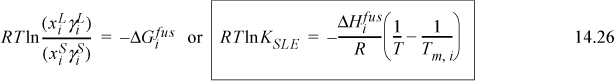
Let us consider a practical example of dissolving naphthalene (2) in n-hexane (1) at 298 K. Since the normal melting temperature for pure naphthalene is 353.3 K, how can we explain the phenomenon that the naphthalene dissolves in hexane? First, recall that the naphthalene will dissolve in the n-hexane if the total Gibbs energy of the system (n-hexane and naphthalene) decreases upon dissolution. Thus, more and more solid may be added to the liquid solution until any further addition causes the total Gibbs energy to increase rather than decrease. This method of calculating equilibrium is fairly tedious to apply, and a preferred method is used that gives identical results: The solubility limit is reached when the chemical potential of the naphthalene in the liquid is the same as the chemical potential of the pure solid naphthalene. Therefore, we solve the problem by equating the chemical potentials for naphthalene in the liquid and solid phases.
The equilibrium can be written as ![]() or, recognizing the notational definitions
or, recognizing the notational definitions ![]() and
and ![]() , therefore,
, therefore,
Next, envision the hypothetical pathway shown in Fig. 14.9 to calculate the chemical potential difference given by Eqn. 14.14, which consists of two primary steps.

Figure 14.9. Illustration of the two-step process for calculating solubility of solids in liquids. Overall, ![]() . Note that the Gibbs energy goes up in Step 1 to create liquid, below the normal melting Tm, but the Gibbs energy goes down when the liquid is mixed.
. Note that the Gibbs energy goes up in Step 1 to create liquid, below the normal melting Tm, but the Gibbs energy goes down when the liquid is mixed.
Step 1. Naphthalene is melted to form a hypothetical liquid at 298 K. The Gibbs energy change for this step is positive as discussed above. The Gibbs energy change is:
where the superscript hypL indicates a hypothetical liquid.
Step 2. The hypothetical liquid naphthalene is mixed with liquid n-hexane. If the solution is nonideal, the Gibbs energy change for component 2 is
The Gibbs energy change for this step is always negative if mixing occurs spontaneously, and must be large enough to cancel the Gibbs energy change from step 1.
![]() Solubility is determined by a balance between the positive ΔGfus and the negative Gibbs energy effect of mixing.
Solubility is determined by a balance between the positive ΔGfus and the negative Gibbs energy effect of mixing.
Then clearly, from Fig. 14.9 and Eqns. 14.14 through 14.16,
where T is 298 K for our example. Relations for the activity coefficients in the right-hand side of the equation have been developed in previous chapters. In the next subsection, the calculation of ![]() is explained.
is explained.
Formation of a Hypothetical Liquid
The Gibbs energy change for step 1 is most easily calculated using the entropies and enthalpies. For an isothermal process, we can write:
dG = dH – T dS
Continuing with the example of dissolving naphthalene at 298 K, the Gibbs energy change for melting naphthalene at 298 K can be calculated from the enthalpy and entropy of fusion,
where T = 298 K. ΔH298fus can be calculated by determining the enthalpies of the liquid and solid phases relative to the normal melting temperature, where the heat of fusion, ![]() . The enthalpy of solid at 353.3 K relative to solid at 298 K (step 1(a) of Fig. 14.9) is
. The enthalpy of solid at 353.3 K relative to solid at 298 K (step 1(a) of Fig. 14.9) is
The enthalpy of the liquid at 298 K relative to liquid at 353.3 K (step 1(c) of Fig. 14.9) is:
Thus, the ![]() for melting is
for melting is

which we can generalize to

A similar derivation for the entropy gives

In addition to these relationships, at the normal melting temperature, since ![]() ,
,

where Tm = 353.3 K. Combining the results and neglecting the integrals (which are nonzero, but essentially cancel each other), we have
where for our example, T = 298.15 and Tm = 353.3. This is the ![]() that we desire for Eqn. 14.17.
that we desire for Eqn. 14.17.
Criteria for Equilibrium
In general, combining Eqn. 14.22 with Eqn. 14.17, we arrive at the equation for the solubility of component 2,

where heat of fusion is at the normal melting temperature of 2, and heat capacity integrals are neglected.
Example 14.8. Variation of solid solubility with temperature
Estimate the solubility of naphthalene in n-hexane for the range T = [298, 350K] using the SSCED model. Plot log10(xN) versus 1000/T.
Solution
From Appendix E, Tm,2 = 353.3 K and ΔHfus = 18,800J/mol.
We can begin at 298 K, assuming an ideal solution. Then
xN = exp[(–18800/8.314)·(1/298 – 1/353.3)] = 0.305.
Starting with xN = 0.305 as an initial guess,
ΦN = 0.305·130.6/(0.695·130.3 + 0.305·130.6) = 0.306.
Noting that δ1′ = 14.93, δ2′ = 19.19 and k12 = 0.0052 => γ2 = 1.693.
xN = 0.305/1.693 = 0.1802. Iterating on xN to achieve consistency, xN = 0.135. Repeating this procedure at other temperatures gives Fig. 14.10.

Figure 14.10. Freezing curve for the system n-hexane(1) + naphthalene(2). Experimental data of H.L. Ward, 1926. J. Phys. Chem., 30:1316.
Hexane also dissolves in a hexane–naphthalene solution below its melting temperature. The general relationship for solving SLE can be written as:

where the heat of fusion is for the pure ith component at its normal melting temperature, Tm,i. Note that Eqns. 14.23 and 14.24 may be used to determine crystallization temperatures at specified compositions.
Example 14.9. Eutectic behavior of chloronitrobenzenes
Fig. 14.11 illustrates application to the system o-chloronitrobenzene (1) + p-chlorornitrobenzene (2). The compounds are chemically similar; thus, the liquid phase may be assumed to be ideal, and the activity coefficients may be set to 1. The two branches represent calculations performed from Eqns. 14.23 and 14.24, each giving one-half the diagram. The curves are hypothetical below the point of intersection. This temperature at the point of intersection of the two curves is called the eutectic temperature, and the composition is the eutectic composition.
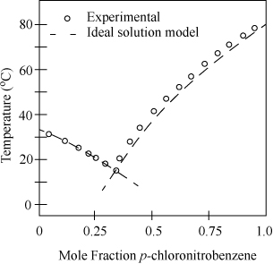
Figure 14.11. Freezing curves for the system o-chloronitrobenzene(1) + p-chloronitrobenzne(2).
Example 14.10. Eutectic behavior of benzene + phenol
In most systems, an activity coefficient model must be included. Fig. 14.12 shows an example where the ideal solution model is not a good approximation, and the activity coefficients are modelled with the UNIFAC activity coefficient model. To solve for solubility given a temperature, the following procedure may be used (taking component 2, for example):
1. Assume the γ2 = 1.
2. Solve Eqn. 14.23 for x2.
3. At this value of x2, determine γ2 from the activity model.
4. Return to step 2, including the value of γ2 in Eqn. 14.23, iterating to converge.

Figure 14.12. Freezing curves for the system benzene(1) + phenol(2). Solid line, UNIFAC prediction; dashed line, ideal solution prediction; squares, Tsakalotos, D., Guye, P. 1910. J. Chim. Phys. 8:340; circles, Hatcher, W., Skirrow, F. J. Am. Chem. Soc., 1917. 39:1939. Based on figure of Gmehling, J., Anderson, T., Prausnitz, 1978. J. Ind. Eng. Chem Fundam. 17:269.
This is a relatively stable iteration, and Excel Solver can iterate on activity by adjusting composition, bypassing the successive substitution method above.
A common procedure when crystallizing products of a pharmaceutical process is to add an antisolvent. The SSCED model is especially convenient for this kind of application because: (1) The concentrations are generally small for crystalline products left in solution; and (2) the infinite dilution activity coefficient of the precipitate involves a simple average of the solvent and antisolvent properties. With these concepts in mind, it is straightforward to tailor a solvent to achieve a target composition at a given temperature.
Example 14.11. Precipitation by adding antisolvent
Ephedrine is a commonly used stimulant, appetite suppressant, and decongestant, related to pseudoephedrine. It can be extracted from the Chinese herb, ma huang. Ephedrine is to be crystallized from ethanol at 278 K by adding water as an antisolvent.
a. Estimate the mole fraction of water needed to reduce the concentration of ephedrine in solution to 0.1mol% using the SSCED model.
b. Yalkowsky and Valvani (1980) have suggested that ΔSfus = 56.5 J/mol-K for rigid molecules.a Evaluate this relation in comparison to the estimated value of ΔHfus = 25kJ/mol.
Additional data for ephedrine are Mw = 165.2; Tm = 313K; and ΔHfus = 25kJ/mol.
a. From Eqn. 14.25, Tm,i = 313 K and ΔHfus = 25,000J/mol. We can begin by solving for the target value of the activity coefficient, noting that the concentration of drug is practically infinitely dilute. Then using xi = 1E-3 to approximate infinite dilution,
The solution requires iteration using Eqn. 12.55. As the mole fraction of water is increased, the activity coefficient of ephedrine increases because water is the antisolvent.
Since we have worked the problem before, “Guessing” a value of x1 = 0.2102,
Φ1 = 0.2102(58.3)/(0.2102·58.3 + 0.7898·18.0) = 0.4627
<δ’> = 0.4627(18.68) + 0.5373(27.94) = 23.66
From Eqn. 12.51,
k12 = 0.0318; k13 = 0.0028; k23 = 0.0571;
=> <k3m> = 0.4627(18.68)0.0028 + 0.5373(27.94)0.0571 = 0.8808;
Similarly, <k1m> = 0.4779; <k2m> = 0.2752;
<<kmm>> = 0.4627(18.68)0.4779 + 0.5373(27.94)0.2752 = 8.262.
By Eqn. 12.55, RTlnγ3 = 172.3((16.36 – 23.66)2 + 2(16.36)0.8808 – 8.262) => γ3 = 245. So the solution should be 79 mol% water. Good “guess!”
b. With ΔSfus = 56.5 and Tm = 313K, ΔHfus = 56.5(313) = 17,700 J/mol, 29% lower than 25,000. The rule does not appear to apply to this compound.
a. Connors, K.A. 2002. Thermodynamics of Pharmaceutical Systems: An Introduction for Students of Pharmacy, Hoboken, NJ: Wiley, p. 129.
A special feature of Example 14.11 is the way it shows how to tailor a solvent to achieve a particular environment for a target solute. A similar approach could be applied to compatibilizing a liquid solvent to avoid LLE. For example, how much methanol should be added to isooctane to reduce the activity coefficient of water below a value of 7.4? This is the calculation behind “dry gas,” used to dissolve water from gas tanks.
SLE with Solid Mixtures
So far, we have only covered phase behavior in systems where the solids are completely immiscible in each other. Fig. 14.13 illustrates a case where the solids form solid solutions, and Fig. 14.14 illustrates behavior where compounds are formed in the solid complexes. Also, the case of wax precipitation from petroleum results in a range of n-C20 to n-C35 straight chain alkanes being mixed in the solid phase. Paraffin wax that you can purchase in the grocery store is primarily composed of n-C20 to n-C35 straight chain alkanes. For the case of liquid and solid mixtures in equilibrium, the derivation of the equilibrium relationship can be modified by adding a step for “unmixing” of solid solutions to the schematic of Fig. 14.9 on page 558. This step is analogous to a reversal of step 2 of the diagram except involving solid solutions and pure solids rather than liquid solutions and pure liquids. For each component in the mixtures:

Figure 14.13. Freezing curves for the Azoxybenzene(1) + azobenzene(2) system illustrating a system with solid-solid solubility. Based on Hildebrand, J.H., Scott, R.L., Solubility of Nonelectrolytes, New York, NY: Dover, 1964.
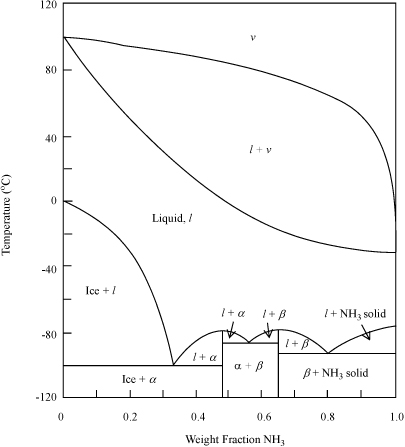
Figure 14.14. Solid-liquid and vapor-liquid behavior for the ammonia(1) + water(2) system at 1.013 bar. NH3 and H2O form two crystals in the stoichiometries: (α) NH3·H2O;(β) 2NH3·H2O. (Based on Landolt-Börnstein, 1960. II/2a:377.)
Thus, we can recognize an SLE K-ratio on the left-hand side, ![]() ,
,
and we can recognize Eqn. 14.24 as a simplification where for a pure solid, ![]() .
.
Petroleum Wax Precipitation
An especially difficult problem in the recovery of natural gas is the clogging of pipes caused by small amounts of wax that accumulate over time. In the Gulf of Mexico, natural gas at the bottom of the well can be 250 bars and 100°C, but it must be reduced to 100 bars to be permitted in the pipeline, and the sea floor can drop to 5°C. The reduction in pressure and temperature results in a loss of carrying power and the small amounts of heavy liquid hydrocarbons can condense, eventually coating the walls with viscous liquid. After the liquid has formed, further cooling can cause solid wax to deposit on the walls of the pipe. These deposits cause constrictions and larger pressure drops that lead to more deposits, and so forth.
Naturally occurring petroleum co-produced with natural gas is a complex mixture of hundreds of individual components. Rather than attempt to specify the identity and composition of every component, it is conventional to collect several fractions of the original according to the ranges of their molecular weights. Hansen et al.2 provide the data in the first four columns of Table 14.1 for the composition, mass density, and molecular weight of several fractions from a typical petroleum stream. This kind of data is typically collected by distilling the initial sample and collecting fractions over time. As the lower molecular weight species are removed, the boiling temperature rises and the distillate collected over each particular temperature range is stored in a separate container. The weight of each fraction relative to the weight of the initial sample gives the composition of that species fraction. The mass of each fraction divided by its volume gives the density. And the average molecular weight can be characterized by gas chromatography or through correlations with viscosity. Note that the molecular weight for any particular species is not necessarily equal to the molecular weight for the corresponding saturated hydrocarbon. This is an indication that olefins, naphthenics, and aromatics are present in significant compositions. The objective of this example problem is to treat the data of Hansen et al. as characteristic of a gas condensate and compute the fractions of the stream that form solids at each temperature.
Table 14.1. Summary of Data for Wax Fractions and Calculations of the Precipitate Composition as Calculated by Example 14.12
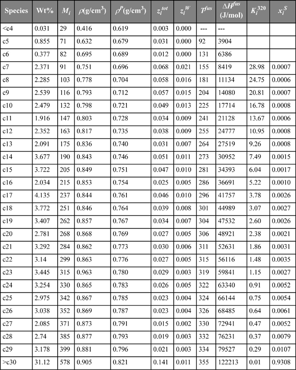
The fusion (melting) temperatures and heats of fusion for n-paraffins can be calculated according to the correlations of Won.3
Noting that each species fraction can contain many species besides the n-paraffins that are responsible for practically all wax formation, it is necessary to estimate the portion of each species fraction that can form a wax. Since the densities of n-paraffins are well known, it is convenient to use the difference between the observed density and the density of an n-paraffin of the same molecular weight as a measure of the n-paraffin content. The correlations for estimating the percentage of wax-forming components in the feed (ziW) are taken from Pedersen.4

where ![]() is the species overall mole fraction in the initial sample.
is the species overall mole fraction in the initial sample.
![]() is the portion of that fraction which is wax-forming (i.e., n-paraffin).
is the portion of that fraction which is wax-forming (i.e., n-paraffin).
Example 14.12. Wax precipitation
Use the data from the first four columns of Table 14.1 and correlations for wax to estimate the solid wax phase amount and the composition of the solid as a function of temperature. Use your estimates to predict the temperature at which wax begins to precipitate. Hansen et al. give the experimental value as 304 K.
Solution
This problem is basically a multicomponent variation of the binary solid-liquid equilibrium problems discussed above. The main difference is that the solid phase is not pure. We can adapt the algorithm as follows.
Assuming ideal solution behavior for both the solid and liquid phases, we define ![]() , and as before, we assume the difference in heat capacities between liquid and solid is negligible relative to the heat of fusion,
, and as before, we assume the difference in heat capacities between liquid and solid is negligible relative to the heat of fusion,
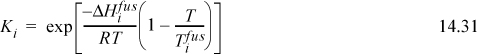
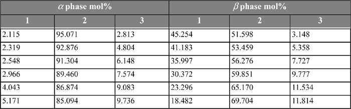
which is independent of the compositions of the liquid and solid phases because of the ideal solution assumptions. The solid solution mole fraction is given by ![]() . Compare this method to the vapor-liquid calculations using the shortcut K-ratio in Chapter 9. This is a liquid-solid freezing temperature analog to the vapor-liquid dew-temperature procedure. The liquid mole fractions are given by the ziW values in the table below. All that remains is to guess values of T, which changes all Ki until
. Compare this method to the vapor-liquid calculations using the shortcut K-ratio in Chapter 9. This is a liquid-solid freezing temperature analog to the vapor-liquid dew-temperature procedure. The liquid mole fractions are given by the ziW values in the table below. All that remains is to guess values of T, which changes all Ki until ![]() . Hand calculations would be easy with a couple of components, but spreadsheets are recommended for a multicomponent mixture. Using Solver for spreadsheet Wax.xlsx distributed with the textbook software gives T = 320.7 K. Intermediate results are tabulated in Table 14.1. The T is slightly higher than the experimental value, but reasonably accurate considering the complex nature of the petroleum fractions and their variabilities from one geographic location to another.
. Hand calculations would be easy with a couple of components, but spreadsheets are recommended for a multicomponent mixture. Using Solver for spreadsheet Wax.xlsx distributed with the textbook software gives T = 320.7 K. Intermediate results are tabulated in Table 14.1. The T is slightly higher than the experimental value, but reasonably accurate considering the complex nature of the petroleum fractions and their variabilities from one geographic location to another.
Solid-Liquid Equilibria Summary
Phase equilibrium involving solids is an extension of previous modeling concepts. Like liquid-liquid equilibria, the condensed phase fugacities are quite insensitive to pressure, so the partition coefficients are simply functions of temperature. The main difference is that the heats of fusion are used to relate the component fugacities in their various states of matter. In multicomponent mixtures, the solid-liquid procedures for calculation are analogs of the vapor-liquid procedures, where the partition coefficients are calculated in a different manner.
14.11. Summary
The presentations of LLE and SLE have been brief, but have opened a broad new frontier of phase behavior analysis: multiphase equilibrium. You might find it incredible to see how many phases and peculiar behaviors can be observed with just “oil,” water, and special third components known as surfactants. (Soap is an example of a surfactant.) The short introduction here is a branching point that barely scratches the surface of such oleic and aqueous systems.5 Such molecules are more complicated than we can represent with the simple models here because of the way that they organize to make films and micelles. Far down this road you may begin to understand the forces that hold cell membranes and living organisms together. At the more practical engineering level, you should be able to perform preliminary designs of liquid extraction and crystallization equipment with little more thermodynamical background than has been presented here.
This kind of breadth is possible with such short introductions because the fundamentals have been laid out previously. The key equation in both LLE and SLE is familiar from VLE (Eqn. 11.13):
The liquid phases split because the Gibbs excess energy becomes so large that the stability limit is exceeded. In other words, the fugacities are so high that the components must escape each other, even if their volatilities are too low for VLE. An entropic penalty must be paid, but a highly unfavorable energy of interaction may more than compensate. A convenient guideline is,
Suspect LLE if ![]() , in which case
, in which case ![]() is a good initial guess.6
is a good initial guess.6
With this guideline, LLE computation is a simple coincidence that may occur occasionally during VLE computations. To paraphrase Pasteur, its observation presents no problem if we know how to recognize it. The procedure for calculating Gibbs energy is the same as for VLE. The calculation of the phase distributions requires a flash calculation in terms of liquid-liquid K-ratios. But the flash algorithm has been discussed before and liquid-liquid flash calculations are hardly different from vapor-liquid flash calculations. The introduction to the prospect of LLE has reminded us of the need to check for stability, however. We first encountered the concept of stability in contemplating the critical points of pure fluids. With the prospect of multiple phases, we begin to realize the need to explore critical phase behavior in a systematic fashion. We have treated that problem for binary and ternary mixtures but have not generalized to multicomponent systems. The generalization of critical phase behavior requires a fair amount of calculus and matrix manipulation,7 but leads to a much deeper understanding of stability behavior than we have provided here. As a practical matter, activity coefficient models must be used carefully because the precision of the models is usually inferior to that of VLE predictions for the same systems. In particular, the temperature dependence of LLE is usually not predicted well. Frequently, the miscibility increases with temperature more quickly than predicted by the activity coefficients even with more sophisticated models like UNIQUAC or UNIFAC. Temperature-dependent parameters can improve the fit, but have little theoretical basis, making extrapolations more tenuous than for VLE.
Important Equations
For LLE, the key equation comes from setting the two expressions for fiL equal and canceling fio,
The iteration for LLE is a little tricky because it relies on the γ’s being large but they get smaller as the iteration proceeds. If you guess a composition too close to equimolar, you might miss the LLE.
For SLE, the key equation is (Eqn. 14.23),
If γi >> 1 then T → Tm. (It is nonsense if the computations yield a value of T > Tm.) Otherwise, the solubility may be significant at T < Tm. This observation suggests changing the solvent (by adding anti-solvent to increase γi), in addition to simply cooling. This is a common technique in pharmaceutical crystallization, among other applications. SLE computation requires iteration if γi≠ 1, because the liquid composition must be guessed in order to estimate γi. But iterative problems like this are familiar from VLE experience and present no problem.
14.12. Practice Problems
P14.1. It has been suggested that the phase diagram of the hexane + furfural system can be adequately represented by the Margules one-parameter equation, where ln γi = xj2 · 800/T (K). Estimate the liquid-liquid mutual solubilities of each component in each liquid phase at 298 K. (ANS. ~10% each, by symmetry)
P14.2. Suppose the solubility of water in ethyl benzene was measured by Karl-Fisher analysis to be 1 mol%. Use UNIFAC to estimate the solubility of ethylbenzene in the water phase. (ANS. 0.003wt% or 30ppmw)
P14.3. According to Perry’s Handbook, the system water + isobutanol forms an atmospheric pressure azeotrope at 67.14 mol% water and 89.92°C. Based on these data, we can estimate the van Laar coefficients to be A12 = 1.566; A21 = 3.833 at 273 K. Estimate the liquid-liquid mutual solubilities of each component in each liquid phase at 273 K. (ANS. 0.33,0.97)
P14.4. Use the SSCED model to predict the solubility of iodine in carbon tetrachloride at 298 K. Iodine’s melting point is 387 K and Hfus = 15.5 kJ/mol.
14.13. Homework Problems
14.1. Suppose the (1) + (2) system exhibits liquid-liquid immiscibility. Suppose we are at a state where G1/RT = 0.1 and G2/RT = 0.3. The Gibbs energy of mixing quantifies the Gibbs energy of the mixture relative to the Gibbs energies of the pure components. Suppose the excess Gibbs energy for the (1) + (2) mixture is given by:
GE/RT = 2.5 x1 x2
a. Combine this with the Gibbs energy for ideal mixing to calculate the Gibbs energy of mixing across the composition range and plot the results against x1 to illustrate that the system exhibits immiscibility.
b. Draw a tangent to the humps to illustrate that the system is one phase at compositions greater than z1 = 0.854 and less than z1 = 0.145, but will split into two phases with compositions at any intermediate overall composition. Most systems with liquid-liquid immiscibility must be modeled with a more complex formula for excess Gibbs energy. The humps on the diagram are usually off-center, as in Fig. 14.3 on page 545 in the text. The simple model used for the calculations here results in the symmetrical diagram.
c. When a mixture splits into two phases, the over-all fractions (of total moles) of the two phases are found by the lever rule along the composition coordinate. Suppose 0.6 mol of (1) and 0.4 mol of (2) are mixed. Use the lever rule to calculate the total number of moles which would be found in each phase of the actual system. Designate the (1)-rich phase as the β phase.
d. What is the value of the hypothetical Gibbs energy, (expressed as G/RT), of a mixture of 0.6 mol of (1) and 0.4 mol of (2) if the mixture were to remain as one phase? Calculate the Gibbs energy of the total system considering the phase split into two phases, and show that the Gibbs energy is less than the Gibbs energy of the single-phase system.
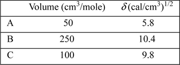
14.2. Assume solvents A and B are virtually insoluble in each other. Component C is soluble in both.
a. Use the Scatchard-Hildebrand theory to estimate the distribution coefficient at low concentrations of C given as (mole fraction C in A)/(mole fraction C in B).
b. If the phase containing A is 0.1 mol% C, estimate the composition of the phase containing B.
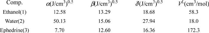
c. If an extractor was designed and constructed, is the distribution coefficient favorable for extraction from B into A? Data:
14.3. A new drug is to have the formula para-CH3CH2-(C6H4)-CH2CH2COOH, where (C6H4) designates a phenyl ring. A useful method for assessing the extent of partitioning between the bloodstream and body fat is to determine the infinite dilution partitioning coefficient for the drug between water and n-octanol. Use UNIFAC to make this determination. The body temperature is 37°C. Will the new drug stay in the bloodstream or move into fatty body parts?
14.4. Use the Scatchard-Hildebrand theory to generate figures of activity as a function of composition and ΔGmix as a function of composition for neopentane and dichloromethane at 0°C. Determine the compositions of the two phases in equilibrium. Data:

14.5. The bubble point of a liquid mixture of n-butanol and water containing 4 mol% butanol is 92.7°C at 1 bar. At 92.7°C the vapor pressure of pure water is 0.784 bar and that of pure n-butanol is 0.427 bar. Assuming the activity coefficient of water in the 4% butanol solution is near unity, estimate the composition of the vapor and activity coefficient of butanol that gives the correct bubble pressure and compare to the values estimated by UNIFAC.
14.6. Schulte et al.8 discuss a linear solvation energy relationship (LSER) method for the partitioning of 41 environmentally important compounds between hexane + water phases at 25°C. The LSER method is based on the idea that contributions to the Gibbs excess energy (and to the logarithm of the partition coefficient) from effects like van der Waals forces and hydrogen bonding are independent of each other. Therefore, these contributions can be added up as separate linear contributions. We can test this hypothesis by plotting partition data for several compounds based on experimental data and LSER. We can also test the predictive capabilities of alternative theories by plotting their results with different curves. Table 14.2 presents the required parameters for the LSER method for several compounds. These parameters are to be substituted into the equation:
Table 14.2. LSER Parameters and Experimental Hexane + Water Partition Coefficients for Several Compounds
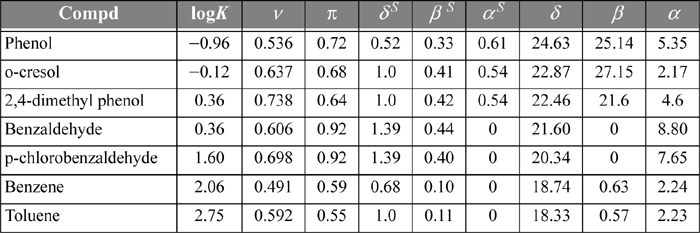
where v = volume parameter, π = polarity parameter, δS = polarizability parameter, βS = hydrogen bond acceptor parameter, and αS = hydrogen bond donor parameter. Compute the log partition coefficients for the following compounds by the LSER method and plot them against the experimental values listed in Table 14.2. Include predictions using the following methods. (Hint: compounds in the environment usually exist at ppm concentrations.)
a. the MAB model.
b. the SSCED model.
c. the UNIFAC model.
14.7. Predict the compositions of the coexisting liquid phases for the system methanol (1) + cyclohexane (2) at 298 K. Let α be the methanol-rich phase.
a. Use the MAB model.
b. Use the SSCED model.
c. Use the UNIFAC model.
14.8. Predict the compositions of the coexisting liquid phases for the system methanol (1) + cyclohexane (2) at 285.15 K and 310.15 K. Let α be the methanol-rich phase. Compare quickly with the data from Fig. 19.12 on page 804 and comment on the accuracy of the results. (Include a printout of your results including converged compositions and activity coefficients of both phases at one of the temperatures.)
a. Use the MAB model.
b. Use the SSCED model.
c. Use the UNIFAC model.
14.9. Benzene and water are virtually immiscible. What is the bubble pressure of an overall mixture that is 50 mol% of each at 75°C?
14.10. Water + hexane and water + benzene are immiscible pairs.
a. The binary system water + benzene boils at 69.4°C and 760 mmHg. What is the activity coefficient of benzene in water if the solubility at this point is xB = 1.6E–4, using only this information and the Antoine coefficients?
b. What is the vapor composition at the bubble pressure at room temperature (292 K) for a ternary mixture consisting of 1 mole overall of each component if the organic layer is assumed to be an ideal solution?
c. What is the vapor composition at the bubble pressure at room temperature (292 K) for a ternary mixture consisting of 1 mole overall of each component if the activity coefficients of the organic layer are predicted by UNIFAC?
The following problems concern LLE in ternary systems. Experimental data for the systems are listed in Tables 14.3 and 14.4.
Table 14.3. Water(1) + Methylethylketone(MEK)(2) + Acetic Acid(3) System at T = 299.85 Ka

a. Skrzec, A.E., Murphy, N.F. 1954. Ind. Eng. Chem. 46:2245.
Table 14.4. 1-Butanol(1) + water(2) + methanol(3) at 288.15 Ka as reported by Mueller
a. Mueller, A.J., Pugsley, L.I., Ferguson, J.B. 1931. J. Phys. Chem. 35:1314.
14.11. Consider the system water(1) + MEK(2) at 299.85 K. The solubilities measured by Skrzec, A.E., Murphy, N.F., 1954. Ind. Eng. Chem., 46:2245, are ![]() and
and ![]() . For a binary system, the LLE iteration procedure has been outlined in Example 14.4. Apply the procedure to determine the mutual solubilities predicted by UNIQUAC. The mixture parameters are r = [0.92, 3.2479], q = [1.40, 2.876], a12 = –2.0882 K, and a21 = 345.53 K. Let phase α be the water-rich phase.
. For a binary system, the LLE iteration procedure has been outlined in Example 14.4. Apply the procedure to determine the mutual solubilities predicted by UNIQUAC. The mixture parameters are r = [0.92, 3.2479], q = [1.40, 2.876], a12 = –2.0882 K, and a21 = 345.53 K. Let phase α be the water-rich phase.
14.12. For a binary system, iterations can be performed by finding a new value of ![]() from only the K-ratios as shown in Eqn. 14.5. For a ternary system, we need at least one composition. Derive the iteration formula, using
from only the K-ratios as shown in Eqn. 14.5. For a ternary system, we need at least one composition. Derive the iteration formula, using ![]() as the specified composition
as the specified composition
14.13. Consider the system water(1) + methylethylketone(MEK)(2) + acetic acid(AA)(3) at 299.85 K. For a ternary LLE system, estimate tie lines at x3α = 0.005, 0.01, 0.02, using UNIQUAC, where the parameter values are r = [0.92, 3.2479, 2.2024], q = [1.40, 2.876, 2.072], and the a values (in K) are a12 = –2.0882, a21 = 345.53, a13 = 254.15, a31 = –301.02, a23 = –254.13, a32 = –4.5537. Let α be the water-rich phase. Plot the results on rectangular coordinates, using x1 as the abscissa and x3 as the ordinate. Connect the tie lines on the plot. Add the experimental tie lines (Table 14.3) to the same plot using different symbols.
14.14. One mole of a stream containing pentane, acetone, methanol, and water in proportions z = 0.75, 0.13, 0.11, 0.01, respectively, is to be mixed and decanted with 1 mol of pure water at 25°C. Estimate the partition coefficients for each of the components and the proportion of lower-phase/Feed where “Feed” includes both the pentane-rich and pure water streams with the specified model.
a. The MAB model.
b. The SSCED model.
c. The UNIFAC model.
14.15. Calculate the LLE in the system 1-butanol(1) + water(2) + methanol(3) at 288.15 K, using UNIQUAC with the following parameters: r = [3.4543, 0.92, 1.4311]; q = [3.052, 1.4, 1.432]; and the a values (in K) are a13 = 355.54; a31 = –164.09; a12 = –82.688; a21 = 443.56; a32 = –85.451; a23 = –321.92; and compare graphically with the data from Table 14.4.
14.16. Solve problem 14.13, except use the specified model.
a. The MAB model.
b. The SSCED model.
c. The UNIFAC model.
14.17. Consider the system water(1) + methylethylketone(MEK)(2) + propanoic acid(PA)(3). Use UNIFAC to predict the compositions for the coexisting phases at x3α = 0.01, 0.05, and 0.10 at 298.15 K. Let α be the water-rich phase. Plot the results on rectangular coordinates by using x1 as the abscissa and x3 as the ordinate. Connect the tie lines on the plot.
14.18. Solve problem 14.15, except use the specified model.
a. The MAB model.
b. The SSCED model.
c. The UNIFAC model.
14.19. Derive the formulas for the spinodal curves of the Flory-Huggins model and plot the spinodals (T versus xα, xβ) of several polystyrenes in cyclohexane using UNIFAC parameters to estimate the volume of polystyrene relative to ethylbenzene and taking the experimental values of solubility parameters and molar volumes for the species when Nd = 1. Take the degrees of polymerization of polystyrene to be 100, 200, 500, 1000. Plot the estimated reciprocal critical temperatures versus Nd–1/2. Mark the infinite molecular weight critical temperature on both plots with a big X.
Solid-Liquid Behavior
14.20. In the treatment of solid-liquid equilibria, the effects of pressure on melting points are neglected.
a. Draw a schematic of the Gibbs energy of liquid and solid phases versus pressure at constant temperature for a compound for which the molar volume of the solid is less than the molar volume of the liquid. Plot both curves on the same figure, and indicate the melting pressure. Most chemicals follow this type of behavior.
b. For water, the molar volume of the solid is greater than the molar volume of the liquid. Sketch the Gibbs energy of liquid and solid phases as a function of pressure at constant temperature for this type of behavior. Plot both curves on the same figure, and indicate the melting pressure.
c. Calculate the hypothetical Gibbs energy for melting solid naphthalene at 5 bar and the normal melting temperature, 80.2°C. You may assume that the liquid and solid are incompressible. Be sure to clearly specify the path you use for your calculation. VL = 124.8 cm3/gmole, VS = 133 cm3/gmole.
d. Calculate the hypothetical Gibbs energy for melting solid naphthalene at 1 atm and 78°C. Compare the magnitude with the results of part (c) to verify that the pressure effects are small relative to temperature effects.
14.21. Generate a solid-liquid equilibrium T-x diagram for naphthalene(1) + biphenyl(2) assuming ideal solutions. What are the predicted eutectic temperature and composition? The experimental eutectic point is 39.4°C and x biphenyl = 0.555 (Lee, H.H., Warner, J.C., 1935. J. Amer. Chem. Soc. 57:318).
14.22. At 25°C, the solubility of naphthalene in n-hexane is 11.9 mol%. The liquid phase is non-ideal. Use the simple solution model GE/RT = Ax1x2 to predict the solubility at 10°C. (The experimental solubility at 10°C is 6.5mol%, Sunier, A. 1930. J. Phys. Chem. 34:2582).
14.23. Phenanthrene and anthracene are structurally very similar. Would you expect them to have similar solubilities in benzene at 25°C? Provide a quantitative answer, and an explanation.
14.24. Predict the solubility (in mole fraction) of phenol at the cited conditions using the specified model. (i) Use the MAB model. (ii) Use the SSCED model. (iii) Use the UNIFAC model.
a. Solubility in n-heptane at 25°C.
b. Solubility in ethanol at 25°C.
c. Solubility in a 50/50 mole ratio of heptane and ethanol at 25°C.
14.25. A 50 wt% (22.5 mol%) solution of ethylene glycol + water freezes at about 240 K.
a. What freezing temperature would be predicted by assuming that ethylene glycol and water form an ideal solution? The freezing occurs by formation of water crystals.
b. Does your calculation indicate that the system has positive or negative deviations from Raoult’s law? Why?
14.26. Determine the ideal solubility of naphthalene in any solvent at 40°C. Then predict the solubility and compare with the experimental solubility (shown in parentheses) for the specified solvent and specified model. (i) Use the MAB model. (ii) Use the SSCED model. (iii) Use the UNIFAC model.
a. Methanol (4.4)
b. Ethanol (7.3)
c. 1-propanol (9.4)
d. 2-propanol (7.6)
e. 1-butanol (11.6)
f. n-hexane (22.2)
g. Cyclohexanol (22.5)
h. Acetic acid (11.7)
i. Acetone (37.8)
j. Chloroform (47.3)
14.27. Determine the ideal solubility of anthracene in any solvent at 20°C. Then predict the solubility and compare with the experimental solubility (shown in parentheses) for the specified solvent and specified model. (i) Use the MAB model. (ii) Use the SSCED model. (iii) Use the UNIFAC model.
a. Acetone (0.31)
b. Chloroform (0.94)
c. Ethanol (0.05)
d. Methanol (0.02)
14.28. Determine the ideal solubility of phenanthrene in any solvent at 20°C. Then predict the solubility and compare with the experimental solubility (shown in parentheses) for the specified solvent and specified model. (i) Use the MAB model. (ii) Use the SSCED model. (iii) Use the UNIFAC model.
a. Acetone (14.5)
b. Chloroform (23.8)
c. Ethanol (1.23)
d. Acetic acid (1.92)
e. Methanol (0.64)
14.29. Determine the solubility curve for naphthalene in the specified solvent, and compare with the literature data:
a. Acetic acid9
b. n-hexane9
c. Cyclohexanol10
d. Acetone9
e. Chloroform11
f. Methanol9
g. n-butanol9
h. Ethanol12
i. n-propanol12
j. 2-propanol12
14.30. The gas condensate from a new gas well in Prudhoe Bay, Alaska has the following weight% of C5, C10, C15, C20, C25, C30, C35, C40, C45, C50, and >C50, respectively: 1, 4, 7, 10, 12, 12, 12, 12, 8, 8, and 14. Estimate the temperature at which wax may begin to precipitate from this liquid.
14.31. Generate an SLE phase diagram for phenol(1) + cyclohexane(2).
a. Assume an ideal solution.
b. Use MAB to model liquid phase nonidealities.
c. Use SSCED to model liquid phase nonidealities.
d. Use UNIFAC to model liquid phase nonidealities.
e. Make a comment about how the solubility of phenol in cyclohexane differs from the solubility in benzene at the same temperature. (See Fig. 14.12 on page 563.)
14.32. Create a flow sheet analog to VLE or LLE calculations to find the melting temperature and liquid phase composition for a given solid mixture composition for the following.
a. Ideal solutions of solid and liquid
b. Nonideal solutions of solid and liquid
14.33. Create a flow sheet analog to VLE or LLE calculations to find the freezing temperature and solid composition for a given liquid composition when the liquids and solids form a non-ideal solution.
14.34. Create a flowsheet analog to VLE or LLE flash calculations to find the coexisting liquid and solid compositions that exist for a liquid-solid mixture of specified overall composition that is between the conditions of first freezing and first melting.
14.35. Salicylic acid is similar in structure to aspirin. Shalmashi et al.13 have measured the data in Table 14.5.
Table 14.5. Solubility of Salicylic Acid in Various Solvents. Compositions in Weight%

a. Find the value of α for salicylic acid in water that best correlates the data, assuming β = 0.
b. Predict the solubility of the acid in ethanol.
c. Plot log(xacid) versus 1000/T including correlated and measured values.
d. Plot all the calculated versus experimental values. This is known as a parity plot.
14.36. Sometimes we would like to enhance the solubility of a drug by adding a cosolvent, instead of adding antisolvent to precipitate. Making optimal use of the data in the previous problem, estimate the amount of ethanol that should be added to water to prepare an aqueous solution of salicylic acid with concentration of 10 wt% at 25°C.
14.37. Yalkowsky and Rubino (1985)14 have observed roughly linear behavior for logarithmic solubility in mixed solvents when plotted as volume fraction of the solvent/cosolvent. That is, log(xi)= Φ1′log(xi,1) + Φ2′log(xi,2) where xi,j is the solubility in the jth pure solvent and Φi′ is the volume fraction on a solute-free basis; for example, ΦE′ = ΦE/(ΦE + ΦW). Use the SSCED model to make your best estimates of the solubility of salicylic acid at 318 K in a range of mixtures with ethanol/water mole fraction ratios of 3/1, 1/1, and 1/3. Plot your results as log10(xacid) versus ΦE′. Include the experimental results and the guideline of Yalkowsky and Rubino. Comment on whether the SSCED model is consistent with the observation of Yalkowsky and Rubino.