
9. Financial Analysis of a Corporation’s Strategic Initiatives
Successful HR strategies are those that align with and support the firm’s business strategy. Successful business strategies are those that create shareholder value. To align a firm’s HR strategy with its business strategy, HR professionals must have at least a basic understanding of the financial models firms use to develop, describe, and evaluate strategic initiatives. That understanding is as important as, or maybe more important than, the ability to use financial models to evaluate operational decisions within the HR function. Recent survey data indicate that approximately 80% of all firms and more than 90% of large firms use discounted cash flow techniques to evaluate strategic investments.1
This chapter has two goals. The first is to demonstrate to HR professionals that they can easily understand enough about these models to be valuable contributors to cross-functional teams using these approaches. The second is to clarify that even when formal modeling is not used, the logic of these models provides an essential framework for thinking about business strategy and the creation of shareholder value. This chapter provides illustrations of models for
• Estimating the NPV of a strategic initiative
• Estimating multiple NPVs using scenario analysis
• Estimating an expected NPV based on judgments about the likelihood of each scenario
• Estimating the NPV when an strategic initiative involves real options
• Estimating the distribution of possible outcomes around an expected NPV
• Calculating the DCF value of a potential acquisition
Estimating the NPV of a Strategic Initiative Such as a New Product Introduction
The logic behind the financial analysis of a strategic investment is, of course, no different than the logic behind the analysis of any other investment. Strategic investment decisions do usually differ in that a larger number of inputs will need to be considered, the amount of risk exposure will be greater, and the consequences of success or failure will be much larger. As an initial example of a strategic investment, consider the introduction of a new product line. Assume your firm is considering producing and marketing a new version of windows. These are energy-efficient, duel casement, out-swing windows for use in new home construction. Exhibit 9-1 is spreadsheet of the type that might be used for modeling this decision. The overall logic of this spreadsheet is to forecast revenues by year, subtract all costs to determine projected profits, and then convert the profit estimates to cash flows. After that is done, it’s straightforward to calculate the NPV and IRR of the proposed product introduction.
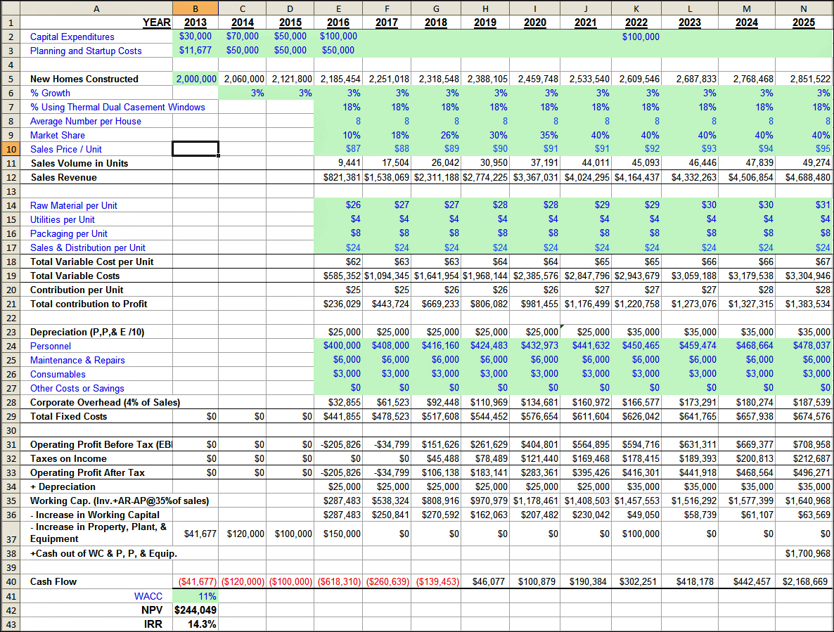
Exhibit 9-1. Estimating NPV and IRR of a strategic initiative
Capital Expenditures and Revenue Forecasts
Rows 2 and 3 of this spreadsheet show the initial capital and planning expenditures that must be made before this new manufacturing facility can be put into operation. Rows 5 through 12 are used to generate a sales forecast. You can begin in cell B5 with government or industry data on the number of new homes currently constructed each year. That number is then increased annually by the estimated growth rates you enter in Row 6. Multiplying the number of homes constructed each year times the Row 7 estimate of the percentage of homes using this type of window times the Row 8 estimate of average number of these windows per house produces an estimate of the industry sales volume in units. Multiplying the industry sales volume by your anticipated market share provides the Row 11 estimate of the number of windows you expect to sell each year. Multiplying the number of windows you expect to sell times the anticipated sales price per window generates the sales revenue projections on Row 12.
Variable Costs and Breakeven Levels
Variable costs are costs that vary with the level of output. In this example, the variable costs are raw materials, utilities, packaging, and sales and distribution costs. Fixed costs are costs that do not vary with the level of output. In this example the fixed costs are property, plant, and equipment (P, P, & E), personnel costs, maintenance and repairs, consumables, and corporate overhead charges. Row 20 shows the contribution to profit per unit. This is calculated as price per unit minus the variable cost per unit. For example, in the year 2016, the sales price of each window (shown on Row 10) is $87, and the total variable cost per window is $62 (shown on Row 18). Therefore, the contribution to profit per window is $25 ($87 – $62). In other words, each window sold covers its own variable cost and provides $25 toward covering the division’s fixed costs. What’s the value in knowing the contribution to profit? You can use that number to calculate the breakeven sales level. If you divide the year 2016 total fixed costs of $441,855 (shown on row 29) by the $25 per window contribution to profit, you see that you must sell 17,674 windows just to cover your fixed costs. This division will be profitable only if sales exceed that number.
Converting Profits Back to Cash Flows
As explained in the previous chapter, your investment decision must be based on the present value of the cash flow in each year, not on the present value of the profits. That is the only way you can answer the question, “Does it make sense to inject cash into this project during the early years to draw out cash in the later years?” The annual profit estimates are not measurements of how much cash will be paid out or received in a given year. To derive the cash flow estimates on Row 40 from the profit estimates on Row 33, you must do three things. Exhibit 9-2 illustrates this process using the data for the year 2019. First, you add back on Row 34 whatever depreciation expense was subtracted out on Row 23. As you know, the annual depreciation expenses are not additional cash outflows but just reallocations for accounting and tax purposes of cash used in earlier periods to purchase long-term assets such as plant and equipment. Second, in any year when you do utilize cash to purchase long-term assets, those amounts are subtracted on Row 37. The third and final step is to subtract on Row 36 the cash used to increase working capital. Working capital is the net amount of cash the firm has tied up in inventories and accounts receivable. Remember that when calculating profit you did not subtract the cost of additions to inventory but only the cost of the windows actually sold in each year. If additional cash were used to build up inventories beyond what was sold that year, we now have to subtract that from the cash on hand. On Row 40, you see that the firm must inject substantial amounts of cash into this venture in the years 2013 to 2018. The cash flows are then projected to become positive in 2019 to 2025. This model, in cell N38, assumes that at the end of year 2025, the firm will cash out the working capital and the property, plant, and equipment invested in this project for $1,700,968. Even if the firm does not actually liquidate these assets, this would be a reasonable way to model the fact that at the end of 2025 this firm will own assets worth $1,700,968.
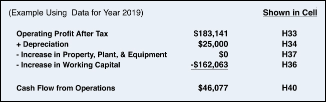
Exhibit 9-2. Converting profits to cash flows
Should You Introduce This New Product Line?
This project requires your firm to inject substantial amounts of cash into this venture in the years 2013–2018 to receive the positive cash flow projected for years 2019 to 2025. If you express all those outflows and inflows in present value terms and then sum them, will this project produce a net gain or a net loss for the shareholders? That is the question answered by the NPV formula in cell B42. That formula is = B40+NPV(B41,C40:N40). If the firm’s weighted average cost of capital is 11% and the cash flow turns out as projected, shareholder value increases by 244,049. An alternative way to evaluate this project would be to calculate its internal rate of return. The formula in cell B43 is =IRR(B40:N40). Remember that the IRR decision rule is that you would proceed with the project only if the IRR is greater than the cost of capital. In this case, the 14% IRR is greater than the firm’s 11% cost of capital, so the project is an attractive one. The NPV in cell B42 was calculated using an 11% discount rate. If the IRR had not been larger than 11%, this NPV would have been negative.
How Useful Are Models of This Type?
A common reaction to models of the type shown in Exhibit 9-1 is that their real-world usefulness is limited by the large number of input assumptions required. It’s true that models of this type are vulnerable to the GIGO (garbage in, garbage out) problem. If your input assumptions are all garbage, the model’s output will be garbage. But think carefully before concluding that is a reason to reject this type of model. There is no assumption that is any more important because you typed it into a spreadsheet than if you made the decision without using a spreadsheet. If whether this initiative is a good idea depends on production costs in year 5, or market share year 2, or interest rates in year 8, you cannot escape that risk reality. Your only choice is to make strategic decisions with or without thinking through the underlying assumptions. Every time you decide to go ahead with a project, you assume that those factors will play out in a way that permits the project’s success. Spreadsheet modeling does not increase the number of assumptions required; it make those assumptions explicit.
There are, of course, a number of potential benefits from the use of models such as the one in Exhibit 9-1. First, they provide guidance as to how you should proceed given your own best estimates of the input factors. Few people, even if they were extremely confident in their estimates of all the input factors shown in Exhibit 9-1, could determine without using a spreadsheet or similar model whether the project would produce a gain or a loss. A second major benefit of making all input assumptions explicit is that they can then be reviewed by your colleagues. If a colleague believes one of your assumptions is too high or too low, it is easy to plug in their estimates instead of yours to determine whether that difference would change the go/no-go policy implications for this project. A third potential benefit from models of this type is the ability to determine which input assumptions are particularly critical and which are of more limited importance. Suppose, for example, you adjust each of the input assumptions up and down by 10%. You might find, for example, that small differences in market share have a much larger impact than small differences in raw materials cost, or you might find the reverse. Identifying which input variables are most critical can help you determine which factors must be studied most carefully during the planning process, and perhaps which factors must be managed most carefully after the project has been implemented.
Models of this type might also assist you in redesigning a strategic initiative. Suppose based on your best assumptions the new initiative you are considering would have a negative NPV. Spreadsheet models of this type may enable you to determine what changes must be made for the project to become an attractive one. How much larger would the selling price need to be? How much lower would the costs need to be? How much larger would our market share need to be? Using spreadsheets it would be easy to answer these and similar questions. You could then determine which, if any, of these changes would be achievable with a project redesign.
Estimating Multiple NPVs Using Scenario Analysis
A natural extension of the previous approach would be to estimate multiple NPVs using scenario analysis. In the previous example, the product was an energy-efficient window used in new home construction. The firm might want to re-estimate the spreadsheet in Exhibit 9-1 under multiple scenarios about how quickly the demand for new homes will grow or how high energy costs will be. Each of these re-estimations would, of course, yield a different potential NPV for this product introduction. The benefit of scenario analysis is that management can now see a range of possible outcomes before making a decision on this project. The limitation of this approach is that it does explicitly incorporate any information about the likelihood of the various scenarios. When judgments can be made about the relative likelihood of alternatives scenarios, it is possible to utilize this information to calculate an expected NPV. An example of that approach is provided in the next section.
Estimating an Expected NPV Based on Judgments About the Likelihood of Each Scenario
Before illustrating the estimation of expected NPVs, it may be useful to review the concept of expected values. Suppose you are playing a casino game that requires you to make a $50 bet. If you win, you get back $100. If you lose, you get back nothing. The casino has designed the game so that on each play you have a 30% chance of winning and a 70% chance of losing. What would your average outcome be if you played that game 1,000 times? With that many plays, you can be relatively confident that you would win approximately 300 times and lose approximately 700 times. You could calculate your average outcome by adding up your winnings (300 × +$100) and your losses (700 × –$50) and dividing by 1,000. You average outcome would be a loss of $5.00 per game. You could do exactly the same calculation more quickly by adding the probability of a win times the amount of a win, plus the probability of a loss times the amount of a loss. In this example that would be (.30 ×$100) + (.70 × –$50) = –$5. Note that if you play this game only once there is no chance that you will lose $5. You will either lose $50 or win $100. The –$5 is an estimate of what the average outcome will be if you play this game many times. Looking at it this way, you can see that expected values are just weighted averages. Each potential outcome is weighted by the probability that it will occur.
You can use this same logic to calculate the expected net present value when there are multiple scenarios describing potential business outcomes. The example in Exhibit 9-3 assumes your firm is considering the introduction of a new cell phone model. Introducing this new phone would have an upfront cost of $100 million. If consumers prefer your phone to the competition, you will in years 1 to 5 receive the positive cash flow shown on Row 2. If consumers prefer the competition over your phone, your firm will experience the negative cash flow shown on Row 3. You could, of course, calculate the NPV for the success scenario and the NPV for the failure scenario. However, if you can make a business judgment about the probabilities of these two scenarios, you can calculate the expected net present value from this product introduction. Your marketing department tells you predicting consumer preferences is difficult and that the new cell phone would have only a 50% probability of success. Using that information you can calculate the expected cash flow shown on Row 5 of the spreadsheet. Each one is calculated by multiplying the probability of success times the cash flow if the product is successful and adding that to the probability of failure times the cash flow if the product is not successful. For example, the year 1 expected cash flow is (.50 × $60) + (.50 × –$40), which is $10. Had you assumed the year 1 probability of success was 70%, the expected cash flow would have been (.70 × $60) + (.30 × –$40), which is $30. Because Row 5 now shows the expected cash flow series, the NPV of this row is the expected NPV of this risky new product introduction. The formula in cell C6 is =C5+NPV(0.12,D5:H5). You would not proceed with the project because the expected outcome is a loss of $40 million. Note that if you introduce this new phone, there is no chance that the expected NPV will result. The project will either be successful or not successful. The expected NPV is an estimate of the average result you would obtain if you made business decisions like this many times. You can improve your organization’s long-run probability of success if you invest only in projects where the expected NPV is positive.
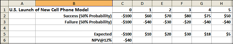
Exhibit 9-3. Calculating the expected NPV when there are multiple scenarios (all dollar amounts in millions)
The NPV When There Are Real Options Like the Ability to Abandon or Expand the Project
The analysis contained Exhibit 9-3 suggests the introduction of the new cell phone would have a negative NPV of $40 million. Obviously, you would not undertake the project if you thought it would reduce shareholder value by $40 million. Perhaps, however, your analysis did not go far enough. If this new product launch goes badly in years 1 and 2, you may be able to withdraw the product and cut your losses. If you believe that is a realistic option, you must adjust the cash flow projections for the failure scenario. Row 2 in Exhibit 9-4 differs from row 2 in Exhibit 9-3 in that the negative cash flow for years 3, 4, and 5 have been replaced with zeros. The assumption is that after the product is withdrawn there will be no more positive or negative cash flows. Changing this scenario changes the expected cash flow series and the expected NPV. The expected NPV from the U.S. launch is now –$9 million, instead of –$40 million. The option to abandon this project if it goes badly was worth $31 million. Of course, you would still not undertake a project with an expected NPV of $–9 million.
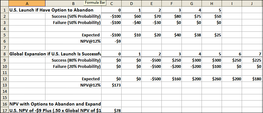
Exhibit 9-4. Calculating the expected NPV when there are options to abandon or expand (all dollar amounts in millions)
There may, however, be an additional option that you should consider. You know that if this project goes badly you can abandon it and cut your losses. But what if the project is a success? Can you expand it and magnify your gains? Suppose that if the U.S. launch of this new phone is successful in years 1 and 2, you will in year 3 introduce it in Europe and Asia. This global expansion option is modeled in Rows 9 and 10 of the spreadsheet in Exhibit 9-4. Because the global expansion will not occur unless the U.S. launch has already proven successful, you might assign a higher success probability to the global launch. The example in Exhibit 9-3 assumes the global launch will have an 80% probability of success. The NPV of the expected cash flow from the global launch is $173 million.
You can now calculate the expected NPV of this new product introduction incorporating both the option to abandon the project if it goes badly and the option to expand it if it goes well. To do this, add the expected NPV of the U.S. launch to one-half of the expected NPV from the global launch. You are including only one-half of the expected NPV from the global launch because it will happen only if the U.S. launch has already been successful and there is only a 50% probability that the U.S. launch will succeed (–9 + .5×173 = 78). Options such as the ability to abandon or expand a project are often referred to as real options to differentiate them from financial options of the type that will be discussed in the next chapter. In this example, had the new product introduction been evaluated without consideration of these real options, the project would have been rejected because its expected NPV was negative. Only when the value of the real options was recognized did it become clear that the expected NPV of the proposal was positive and quite large.
Estimating the Distribution of Possible Outcomes Around an Expected NPV
The previous examples illustrate approaches corporations can use to estimate the expected net present value of a strategic initiative. If possible strategic planners would, of course, like to know more than just the expected NPV from a project under consideration. They would also like to know the distribution of possible NPVs around that expectation. Suppose for example, the most likely NPV from Project A were $10 million and you were confident the actual NPV would fall between $7 million and $13 million. Contrast that with Project B that also has an expected NPV of $10 million, but where the range of possible outcomes is between –$5 million and + $25 million. Even though both projects have the same expected NPV, Project B is a much higher risk. Firms that could not tolerate the possibility of a $5 million loss would need to rule out Project B entirely. Having estimates of the distribution potential investment outcomes can be extremely helpful to those contemplating high-risk business strategies.
All firms making risky investments must consider both the most likely outcome and the range of possible outcomes. Some firms find it useful to develop formal models to estimate those items. The pharmaceutical industry is one that makes large, high-risk investments. Large pharmaceutical companies spend $4 to $8 billion per year per firm on research and development. Ninety-five percent of the projects they initiate end up at a dead end; that is, they do not result in an FDA approvable drug. Because the stakes are so high and the risks are so large, that industry has devoted substantial effort to developing models for assessing the risk associated with strategic investments. Hopefully reviewing the pharmaceutical industry example shown in Exhibit 9-5 demonstrates just how generic these models are and that they can be utilized by firms in most industries.
The spreadsheet reproduced in Exhibits 9-5a and 9-5b describes a strategic choice faced by large pharmaceutical firm. The choice is whether to in-license, that is, license the rights to, a new drug for treating type II diabetes. Rows 1 through 25 of this spreadsheet are shown in Exhibit 9-5a. The approach used to generate the revenue forecasts is similar to the approach used in Exhibit 9-1, so there is probably no need to review each of the steps. It starts with the estimate that 24.5 million people in the United States had type II diabetes in the year 2010. The assumptions shown are then used to calculate the revenue that year. The formula in cell E20 is =+E3*E6*E8*E10*E12*E14*E16*E18. The same approach was used to estimate revenue in each of the other years. The second half of this spreadsheet is shown in Exhibit 9-5b. Rows 27 to 42 contain estimates of the variable and fixed costs to manufacture and sell this drug. The deal costs are shown on Row 44. To in-license this drug would require an upfront payment of $100 million in 2010 and then additional milestone payments in the years 2013 to 2020. With this information you can calculate the after-tax profit shown on row 50. Then using the same logic described earlier, you convert the profit estimates to cash flow estimates. The cash flow is shown on Row 56. The NPV of the proposed deal is shown in cell B58 where the formula is =+B56+NPV(B57,C56:L56). The IRR for this project is shown in cell B59 where the formula is =IRR(B56:L56). The NPV is positive ($188.6 million), and the IRR is greater than the weighted average cost of capital. Both measures suggest this is a project worth pursuing.
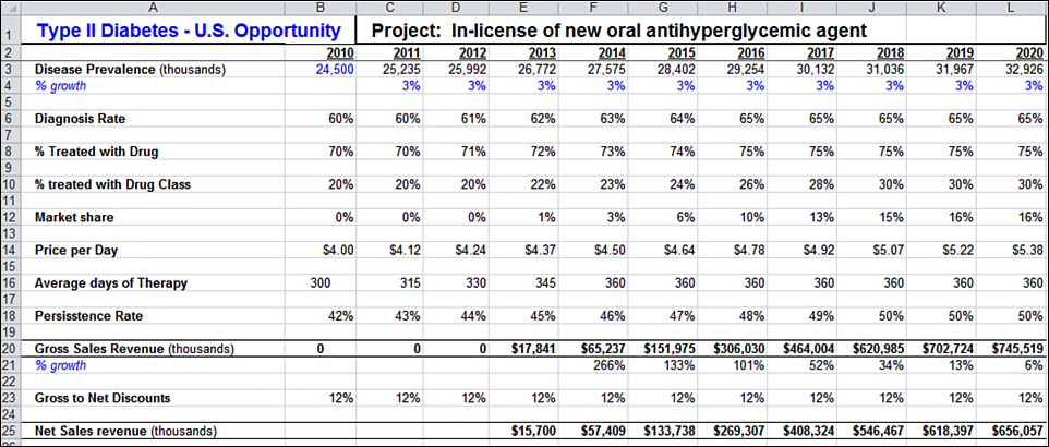
Exhibit 9-5a. Monte Carlo simulation of a strategic initiative
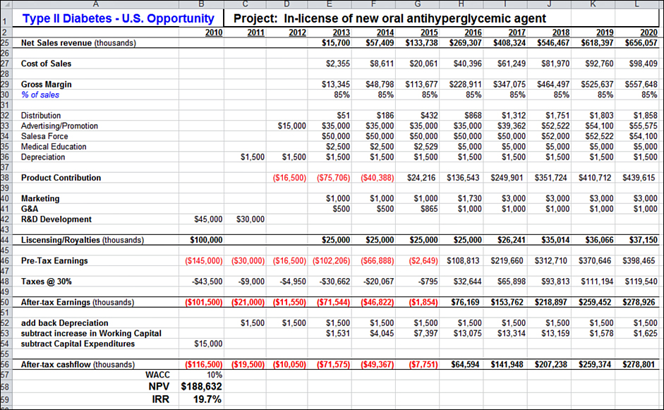
Exhibit 9-5b. Monte Carlo simulation of a strategic initiative (second half)
Using the Spreadsheet to Structure the Deal
Before expanding this model to include a Monte Carlo simulation, look at how it could be used to help negotiate the proposed drug in-licensing. Suppose you are on the team deciding whether to in-license this drug. The firm you are negotiating with feels the terms you have offered, and shown on Row 44, are not sufficiently generous. How attractive would this deal be for your firm if you increased your offer by $10 million? The answer depends heavily on how you structure the payments. Reducing the initial year 2010 payment by $50 million and increasing the year 2020 payments by $60 million would increase your total payments by $10 million. What impact would those changes have on the NPV of this deal? Exhibit 9-5c reveals that entering this altered payment series into Row 44 of the spreadsheet would increase your NPV from $188,632,000 to $207,439,000. Offering to pay an additional $10 million but restructuring the payment sequence would increase your firm’s net benefit by almost $19 million. How is that possible? It is a consequence of the time value of money. In this hypothetical you moved a $50 million payment from 2010 to 2020. If the firm’s weighted average cost of capital is 10% each year that the firm does not have to come up with this $50 million, the firm saves $5 million ($50 million × 10%). Those savings more than offset the present value of the extra $10 million added in year 2020.
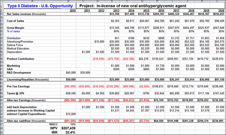
Exhibit 9-5c. Impact on NPV of restructuring licensing and royalty payments
Using Monte Carlo Simulations to Model Risk and Uncertainty
If your estimate for each of the input variables is correct, the proposed drug in-licensing deal will produce a large net benefit for your firm. Of course, there’s almost no chance that all your estimates are correct. It has been said that whenever you make a cash flow forecast, you know you are wrong. You just don’t know by how much or in which direction. Monte Carlo simulation is a technique that can be used to model the uncertainty in your forecasts and to assess the implications of this uncertainty. When Monte Carlo simulations are applied to spreadsheets such as the one in Exhibit 9-5, you have the option to enter into each input cell not just your best estimate but also information about the possible distribution around that estimate. For example, in cell F14 of this spreadsheet, the year 2014 price per dose for this drug is shown as $4.50. Assume that number was the best estimate that your marketing team could provide. However, when pressed they acknowledged that it was only an estimate and that the actual price might be above or below that. If further questioning revealed that they believed the price could be $3.50, $4.50, or $5.50, you could then ask them for their judgments about how likely it was that each of these prices would occur. Suppose their judgment is that there is a 30% chance the price will be $3.50, a 50% chance the price will be $4.50, and a 20% chance the price will be $5.50. How can their judgments about the likelihood of each of the different prices be incorporated into a spreadsheet? Before discussing software for doing that, review what you are trying to achieve.
Suppose you take 10 scraps of paper. On three of them you write $3.50. On five you write $4.50, and on two you write $5.50. You then put all 10 pieces of paper into your desk drawer. You could now recalculate the spreadsheet in Exhibit 9-5 with one difference. When you get to cell F14, you reach into your desk drawer and without looking randomly pull out one of the pieces of paper. Whatever price is on that piece of paper is the number you plug into cell F14. If you did that once, the resulting NPV would be meaningless. However, suppose you repeated that exercise 1,000 times and recorded the 1,000 NPVs that resulted. You could now plot those 1,000 NPVs on a graph and observe both the range of possible NPVs and the frequency with which each NPV occurred. That is in essence what a Monte Carlo simulation does. You could replicate that process in the cells with the price for each of the other years. Actually, you could apply a similar process in any or all of the almost 200 input cells in Exhibit 9-5. Assume you identified 50 key input cells where you thought it was important to consider not just information about the most likely value but also information about the range of possible values. If you were doing this manually, you would need to make a random draw from each of 50 different distributions, plug in those values, and then calculate the first NPV. Make a second draw from each of those 50 distributions, calculate the second NPV, and so on. To repeat that process 1,000 times would be tedious and slow. Fortunately, there is software available that can perform equivalent analyses quickly and simply.
Several companies sell Monte Carlo simulation software that works as an Excel add-in. When this software runs, you have the option to enter into any spreadsheet cell either a specific value or information about the distribution of possible values. The distribution information can be entered in a variety of formats. You could, as in the previous example, enter three prices and estimates of the probability that each of those prices will occur. You could specify a normal distribution by providing the mean and standard deviation. You could specify a distribution that is skewed left or skewed right, or truncated at a particular minimum and/or maximum value. Because these software packages provide a graphical image of the distribution you have specified, using them does not require a mathematics background. When you start the simulation, the software evaluates the spreadsheet 1,000 times (or whatever number of times you specify). Each time, for any cells in which you have specified a distribution, it makes a random draw from that distribution. It then plots the 1,000 NPVs in a graph similar to the one shown in Exhibit 9-6.
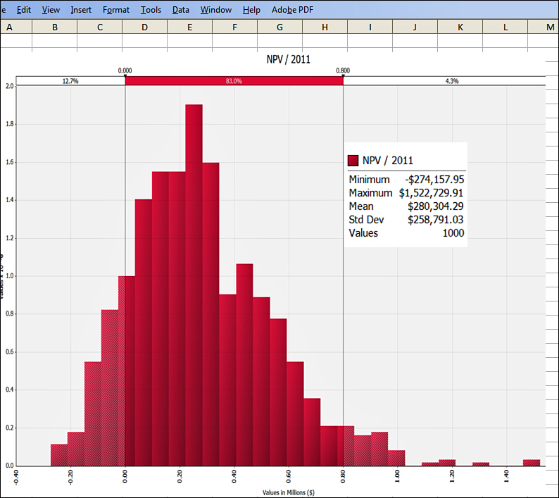
Exhibit 9-6. Output from Monte Carlo simulation showing range of possible NPVs
Interpreting the Output from a Monte Carlo Simulation
You use a simulation like this when you are concerned about the uncertainty of key assumptions. You don’t know whether when you implement this project each of those factors will turn out to be close to what you assumed, or perhaps more favorable or less favorable for the success of the project. Most of the time most of the factors will have values close to their expectation. However, it is possible that all or most of the factors could turn out to be much less favorable than anticipated causing the project to have a much lower than expected NPV. On the other hand, all or most the factors could turn out to be much more favorable than anticipated causing the project to have a much higher than expected NPV. Monte Carlo simulation gives you a way to estimate the magnitude and likelihood of these extreme outcomes. It attempts to answer the questions, “What would the distribution of NPVs be if you undertook projects like this one many times? What would be the average outcome? How much could you lose if things go badly, and what is the likelihood of that? How much could you make if things go well, and what is likelihood of that?”
Exhibit 9-6 is a plot of the NPV value in cell B58 from each of 1,000 independent recalculations on the spreadsheet shown in Exhibit 9-5. In each recalculation when Excel reached a cell where a distribution rather than a single value had been entered, the Monte Carlo add-in made a random draw from that distribution, and the resulting value was used in the spreadsheet calculation. It is exactly analogous to your reaching into your desk drawer and randomly picking one of those 10 scraps of paper to determine which price to plug in to the spreadsheet. In this example, you see that the mean NPV from those 1,000 recalculations of the spreadsheet was $280,304,000. This suggests that if your company made business investments like this many times, you would have an average net benefit of approximately $280 million. In that sense, this project is an attractive one. However, the simulation results also revealed a wide distribution around that average. The largest NPV that occurred during those 1,000 trials was $1,522,730. The smallest NPV was a loss of $274,158. The percentages on the top row of the graph show that the NPV was below zero; that is, the company lost money in 12.7% of those 1,000 trials. A large company that makes many such investments might approve projects such as this because on average they would produce a net gain. A small company making only one such investment might choose to reject it to avoid exposing itself to a 12.7% chance of losing money.
Using DCF to Analyze Mergers and Acquisitions
Discounted cash flow techniques similar to the ones illustrated in the previous examples can be used to estimate the value of a potential acquisition. As in the previous examples, the most challenging part of the process is estimating the future cash flow. Even with a detailed knowledge of the firm to be acquired, its business strategy, its markets, its cost structure, and its competitors, it is difficult to estimate future cash flow. Nevertheless, most buyers use both discounted cash flow models and comparables to estimate the maximum purchase price they should offer. The use of comparables involves comparing the target company to similar companies whose stock is publicly traded or have been acquired recently. If a comparable company’s P/E ratio (stock price divided by earnings per share) was, say, 14, that would imply that its market cap (the value of its outstanding stock) is 14 times its net income. You might then conclude that the appropriate price to pay for the target company is an amount equal to 14 times the target company’s net income. In addition to price to net income, other comparable measures that might be used include a price to EBIT, price to EBITDA, price to sales, price to book value of assets, and price to book value of equity. The two major challenges in using the comparables approach are, of course, identifying companies that are sufficiently similar to the acquisition target and deciding which comparables measure to use. Because using different measures can produce widely varying estimates of the value of a target company, a common approach is to value the target company using multiple comparables measures and discounted cash flow analysis.
An example of using discounted cash flow analysis to evaluate a potential acquisition is shown in Exhibit 9-7. The spreadsheet reproduced in this exhibit assumes that an analysis is being done in the year 2012 for an acquisition that would take place at the beginning of 2013. Rows 6 through 13 contain the forecasts of sales, expenses, and profits for the years 2013 to 2020. Following exactly the same process and logic that was discussed in the earlier capital budgeting examples, you must convert the profit estimates to cash flow estimates. On Row 14, the depreciation expense is added back because it does not represent a cash outflow in that year. On Row 15 and Row 16, any cash used to expand property plant and equipment and to increase the firm’s working capital are subtracted. The resulting cash flow is shown on Row 17.
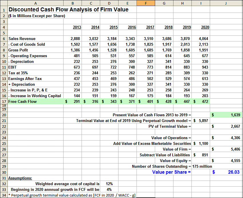
Exhibit 9-7. Using DCF analyses to evaluate mergers and acquisitions (M&A)
Dividing Cash Flows into an Initial Time Horizon and a Terminal Value
Theoretically, the value of a company is the present value of all future cash flow. However, when estimating the value of a potential takeover target, a common approach is to estimate the present value of cash flow over an initial time horizon of 5 to 15 years and then add to that an estimate of what the company will be worth at the end of that initial time horizon. That estimate of what the company will be worth at the end of the initial time horizon is referred to as the terminal value. The assumption is that during this initial time horizon the company driven by its new owners will be undergoing change and that a specific forecast of the cash flow for each year is warranted, but that by the end of this time horizon the company will have reached a steady-state and that cash flow will begin to grow at a constant rate. Selecting the right time horizon is difficult and is just one of the practical problems faced when trying to apply DCF models. Recent survey data indicates that almost one-half of all firms (46%) discount an explicit cash flow forecast for the first 5 years and then add to that an estimate of the terminal value. Just more than one-third (34%) reported using a 10-year explicit forecast period, and only 4% incorporated a specific forecast for 20 years of more.2 The spreadsheet in Exhibit 9-7 treats the years 2013 to 2019 as the initial time horizon and the year 2020 as the estimate of the steady-state condition. The present value of the cash flow in 2013 to 2019 is calculated in cell J20. The formula in that cell is =NPV(D32,B17:H17). D32 is a reference to the cell where the weighted average cost of capital is located.
Which Cost of Capital Should Be Used?
Firms do not typically use their own WACC when valuing a potential acquisition. To more accurately reflect the risk level associated with the target company, it is common to use the target company’s cost of capital or the cost of capital for a group of companies comparable to the target company.
Present Value of a No-Growth Perpetuity
The terminal value at the end of 2019 is calculated in cell I20. The terminal value is estimated as what the finance literature sometimes referred to as a perpetuity. A perpetuity is a perpetual or never-ending annuity. If you assume a no-growth perpetuity, that is, that the cash flow this firm was generating in 2020 would continue unchanged for the indefinite future, the present of that series value could be calculated using this formula:
Present value of a fixed perpetuity = annual cash flow / discount rate
You may feel it is counterintuitive to put a finite value on an infinite series of payments, but perhaps the following example will make this seem more reasonable. How much would you pay for the right to receive $10,000 per year forever? Suppose you put $100,000 in a bank account paying 10% and instructed that bank to send you your interest at the end of each year and roll over the principal to the next year. For a single $100,000 payment, you could receive $10,000 per year forever. That is assuming the bank continued to exist and to follow your instructions, and that 10% continued to be the correct interest rate. Applying the perpetuity formula you see that at a discount rate of 10% the present value of a cash flow $10,000 per year forever is $10,000/.10 or $100,000.
Present Value of a Growth Perpetuity
In this example is it unrealistic to assume that cash flow would remain indefinitely at the year 2020 level. If you can estimate the rate at which these cash flows grow, you can calculate the present value of a growth perpetuity using this formula:
Present value of a growth perpetuity = annual cash flow / (discount rate – growth rate)
Subtracting the growth rate from the discount rate makes the denominator of this fraction smaller, and therefore the present value is larger. The larger the assumed growth rate, the greater the present value of this cash flow series. The formula in cell I20 of this spreadsheet is =+I17/(D32-D33). That formula divides the 2020 cash flows of $472 million by the 12% weighted average cost of capital minus the 4% growth rate. The result is an estimate that at the end of 2019 this firm’s value will be $5.897 billion. Because that is the value at the end of 2019, you need to convert it to today’s present value by dividing by (1+i)t. The formula in cell J22 is =I21/(1+D32)^7. The Excel symbol for exponentiation, raising a number to a power, is ^. A recent survey of corporate financial professionals revealed that the perpetuity growth model is the approach most frequently used to estimate the terminal or continuing value of a project or other strategic investment.3 The present value of this firm’s business operations is therefore estimated in cell J24 to be $4.306 billion. That is the sum of present value of the cash flows during the initial time horizon (cell J20) and the present value of the terminal value (cell J22). If this firm has cash or marketable securities in an amount greater than what is needed to support the firm’s business operations, this excess cash represents additional real value to the acquirer. When this amount is added to the value of the firm’s operations, you see that the value of the firm is $5.406 billion. Firm value minus liabilities is the value of the equity in this firm. Dividing the $4.555 billion equity value by the number of shares of stock outstanding yields a price per share of $26.03. Acquisitions are, of course, a negotiation process, and $26.03 per share is the maximum that one would pay. The initial offer would almost certainly be much below that.
Stand-Alone Value Plus Synergies Minus Deal Costs Equals Acquisition Value
The previous example considered only the stand-alone value of the potential acquisition. Anticipated synergies between the purchasing company and the acquired company are often a primary motivation for undertaking an acquisition. Synergies may increase revenues and/or decrease costs. The acquired company’s sales may increase because its products are now marketed through the distribution networks of the purchasing company or because they benefit from association with the purchasing company’s brand. The sales of the purchasing company might increase because the products of the acquired company fill out its product line providing greater access to those customers who prefer a full-service vendor. Cost reductions can result from economies of scale. The combined firms may not need two full scale finance departments, HR departments, IT departments, and so on. These cost-reducing restructurings can, of course, be difficult for the individuals involved even when they make the combined organization more efficient. In addition to improving cash flow, acquisitions also have the potential to decrease the riskiness (volatility) in the cash flow of the combined firm. Having a diversified portfolio of products will reduce volatility by the greatest amount when the cash flow from different products are negatively correlated. For example, aggregate cash flow volatility is reduced if the firm has some products that do well when energy prices are high and other products that do well when energy prices are low.
The spreadsheet reproduced in Exhibit 9-8 illustrates that an acquisition’s value is its stand-alone value plus the value of synergies achieved, minus the price paid and related deal costs. This summary spreadsheet utilizes stand-alone and synergy cash flow projections that were estimated through a process similar to that described in Exhibit 9-7. The synergy cash flow is negative in the first year because substantial one-time restructuring costs were anticipated. Unlike the example in Exhibit 9-7 where the transaction involved purchasing the stock of the acquired company, this example assumes the assets within one division of a corporation are being purchased. In an asset purchase, the purchasing firm does not assume responsibility for the liabilities of the division or company being acquired. This spreadsheet models a $4 billion purchase price plus $120 million in deal costs spread over 3 years. The net present value of the cash flow shown on Row 10 is calculated in cell B12. The approach is exactly the same as the one used in Exhibit 9-7. The formula in cell B12 is =NPV(C16,B10:H10)+(I10/(C16-C17)). If all these assumptions turned out to be correct, the acquisition would add $740 million in shareholder value.
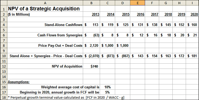
Exhibit 9-8. The pursuit of synergies can motivate M&A activity.
Weak Assumptions or Weak Execution?
Unfortunately, the empirical evidence suggests most acquisitions don’t create much, if any, value for the acquiring company’s shareholders. A study by the consulting firm McKinsey and Company looked at 1,415 acquisitions from 1997 through 2009. Its conclusion was that roughly one-third created value, one-third did not, and for the final third, the empirical results were inconclusive.4 Why do so many acquisitions fail to achieve the benefits projected by models such as the ones previously illustrated? It’s not because of flaws in the logic of these models. It’s because either the assumptions plugged into these models were unrealistic or firms could not execute on the activities required to achieve these outcomes. Estimating a target company’s current worth is always difficult, and projecting the synergies an acquisition will create is even more problematic. Cost reduction synergies may be relatively easy to quantify and deliver. Sales growth synergies are harder to project and attain. An acquisition that would not make economic sense without the projected synergies is a high-risk acquisition.
HR managers in their strategic partner role can greatly influence the likelihood that M&A activity leads to true value creation. HR’s initial point of influence is in the design of a compensation system that rewards managers for pursuing value creating acquisitions without encouraging them to take excessive risks. This challenge is discussed in Chapter 12, “Creating Value and Rewarding Value Creation.” HR plays a key role during the due diligence phase of the acquisition planning. Determining the value of the targeted company’s workforce is an essential task that most investment bankers are unqualified to perform. Projecting the workforce restructuring costs and synergies is also an area in which substantial input from HR managers will be needed. Post-merger HR must, of course, play a central role in the merging of the workforces, systems, and cultures. This last step can be the primary determinant of whether an acquisition succeeds or fails. To function in these critical roles, HR managers must understand the firm’s business strategy, the acquisition strategy, and the basics of the financial models used to evaluate the acquisition. This chapter has provided illustrations of the types of models you are likely to encounter. HR managers should not underestimate their ability to understand these models and to contribute to discussions of M&A plans or other strategic initiatives. Constructing these models will be done by the finance group. It has the easy job. The difficult task is determining the correct assumptions to plug in to these models. That’s an area in which HR can make a huge contribution.