Chapter 12

Composite Objects

Chapters 6 through 11 presented algorithms working on collections of objects (data structures) through iterators or coordinate structures in isolation from construction, destruction, and structural mutation of these collections: Collections themselves were not viewed as objects. This chapter provides examples of composite objects, starting with pairs and constant-size arrays and ending with a taxonomy of implementations of dynamic sequences. We describe a general schema of a composite object containing other objects as its parts. We conclude by demonstrating the mechanism enabling efficient behavior of rearrangement algorithms on nested composite objects.

12.1 Simple Composite Objects

To understand how to extend regularity to composite objects, let us start with some simple cases. In Chapter 1 we introduced the type constructor pair, which, given two types T₀ and T₁, returns the structure type pair_{T0, T1}. We implement pair with a structure template together with some global procedures:

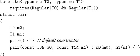
C++ ensures that the default constructor performs a default construction of both members, guaranteeing that they are in partially formed states and can thus be assigned to or destroyed. C++ automatically generates a copy constructor and assignment that, respectively, copies or assigns each member and automatically generates a destructor that invokes the destructor for each member. We need to provide equality and ordering manually:

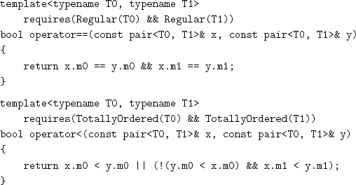
Exercise 12.1 Implement the default ordering, less, for pair_{T0, T1}, using the default orderings for T0 and T1, for situations in which both member types are not totally ordered.

Exercise 12.2 Implement triple_{T0, T1, T2}.

While pair is a heterogeneous type constructor, array_k is a homogeneous type constructor, which, given an integer k and a type T, returns the constant-size sequence type array_k_{k, T}:

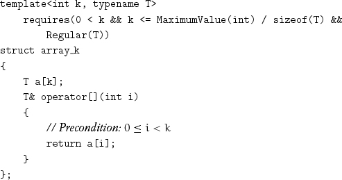
The requirement on k is defined in terms of type attributes. MaximumValue(N) returns the maximum value representable by the integer type N, and sizeof is the built-in type attribute that returns the size of a type. C++ generates the default constructor, copy constructor, assignment, and destructor for array_k with correct semantics. We implement the member function that allows reading or writing x[i].^[1]

IteratorType(array_k_{k, T}) is defined to be pointer to T. We provide procedures to return the first and the limit of the array elements:^[2]

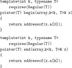
An object x of array_k_{k, T} type can be initialized to a copy of the counted range with code like

copy_n(f, k, begin(x));

We do not know how to implement a proper initializing constructor that avoids the automatically generated default construction of every element of the array. In addition, while copy_n takes any category of iterator and returns the limit iterator, there would be no way to return the limit iterator from a copy constructor.

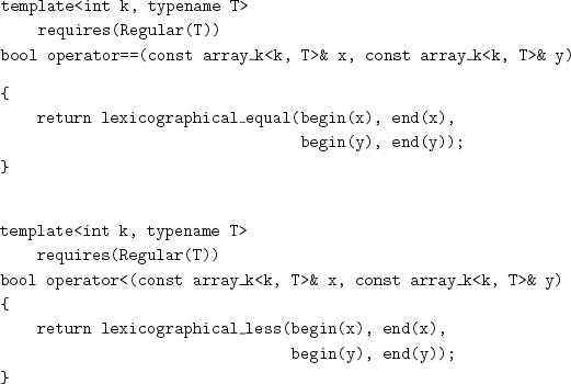
Equality and ordering for arrays use the lexicographical extensions introduced in Chapter 7:

Exercise 12.3 Implement versions of = and < for array_k_{k, T} that generate inline unrolled code for small k.

Exercise 12.4 Implement the default ordering, less, for array_k_{k, T}.

We provide a procedure to return the number of elements in the array:

template<int k, typename T>
    requires(Regular(T))
int size(const array_k<k, T>& x)
{
    return k;
}

and one to determine whether the size is 0:

template<int k, typename T>
    requires(Regular(T))
bool empty(const array_k<k, T>& x)
{
    return false;
}

We took the trouble to define size and empty so that array_k would model Sequence, which we define later.

Exercise 12.5 Extend array_k to accept k = 0.

array_k models the concept Linearizable:

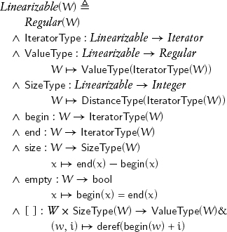
empty always takes constant time, even when size takes linear time. The precondition for w[i] is 0 ≤ i ≤ size(w); its complexity is determined by the iterator type specification of concepts refining Linearizable: linear for forward and bidirectional iterators and constant for indexed and random-access iterators.

A linearizable type describes a range of iterators via the standard functions begin and end, but unlike array_k, copying a linearizable does not need to copy the underlying objects; as we shall see later, it is not a container, a sequence that owns its elements. The following type, for example, models Linearizable and is not a container; it designates a bounded range of iterators residing in some data structure:

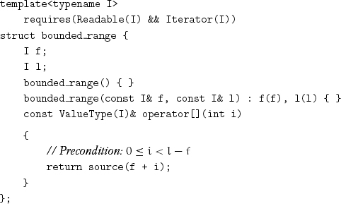
C++ automatically generates the copy constructor, assignment, and destructor, with the same semantics as pair_{I, I}. If T is bounded_range_I, IteratorType(T) is defined to be I, and SizeType(T) is defined to be DistanceType(I).

It is straightforward to define the iterator-related procedures:

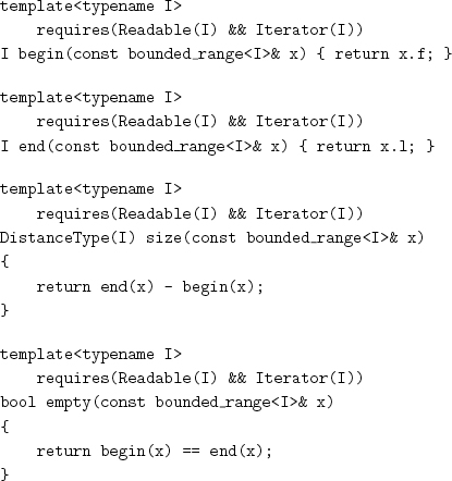
Unlike array_k, equality for bounded_range does not use lexicographic equality but instead effectively treats the object as a pair of iterators and compares the corresponding values:

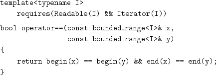
The equality so defined is consistent with the copy constructor generated by C++, which treats it just as a pair of iterators. Consider a type W that models Linearizable. If W is a container with linear coordinate structure, lexicographical_equal is its correct equality, as we defined for array_k. If W is a homogeneous container whose coordinate structure is not linear (e.g., a tree or a matrix), neither lexicographical_equal nor range equality (as we defined for bounded_range) is the correct equality, although lexicographical_equal may still be a useful algorithm. If W is not a container but just a description of a range owned by another data structure, range equality is its correct equality.

The default total ordering for bounded_range_I is defined lexicographically on the pair of iterators, using the default total ordering for I:

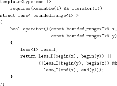
Even when an iterator type has no natural total ordering, it should provide a default total ordering: for example, by treating the bit pattern as an unsigned integer.

pair and array_k are examples of a very broad class of composite objects. An object is a composite object if it is made up of other objects, called its parts. The whole–part relationship satisfies the four properties of connectedness, noncircularity, disjointness, and ownership. Connectedness means that an object has an affiliated coordinate structure that allows every part of the object to be reached from the object’s starting address. Noncircularity means that an object is not a subpart of itself, where subparts of an object are its parts and subparts of its parts. (Noncircularity implies that no object is a part of itself.) Disjointness means that if two objects have a subpart in common, one of the two is a subpart of the other. Ownership means that copying an object copies its parts, and destroying the object destroys its parts. A composite object is dynamic if the set of its parts could change over its lifetime.

We refer to the type of a composite object as a composite object type and to a concept modeled by a composite object type as a composite object concept. No algorithms can be defined on composite objects as such, since composite object is a concept schema rather than a concept.

array_k is a model of the concept Sequence: a composite object concept that refines Linearizable and whose range of elements are its parts:

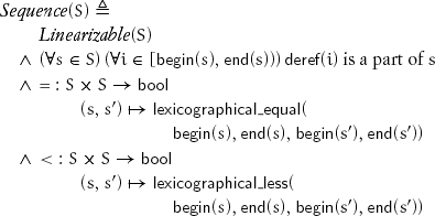
If s and s′ are equal but not identical sequences, begin(s) ≠ begin(s′), but source(begin(s)) = source(begin(s′)). This is an example of projection regularity. Note that begin and end can be regular for a Linearizable that is not a Sequence; for example, they are regular for bounded_range.

Exercise 12.6 Define a property projection_regular_function.

12.2 Dynamic Sequences

array_k_{k, T} is a constant-size sequence: The parameter k is determined at compile time and applies to all objects of the type. We do not define a corresponding concept for constant-size sequences, since we are not aware of other useful models. Similarly, we do not define a concept for a fixed-size sequence, whose size is determined at construction time. All the data structures we know that model a fixed-size sequence also model a dynamic-size sequence, whose size varies as elements are inserted or erased. (There are, however, fixed-size composite objects; for example, n × n square matrices.)

Regardless of the specific data structure, the requirements of regular types dictate standard behavior for a dynamic sequence. When it is destroyed, all its elements are destroyed, and their resources are freed. Equality and total ordering on dynamic sequences are defined lexicographically, just as for array_k. When a dynamic sequence is assigned to, it becomes equal to but disjoint from the right-hand side; similarly, a copy constructor creates an equal but disjoint sequence.

If s is a dynamic-size, or simply dynamic, sequence of size n ≥ 0, inserting a range r of size k at insertion index i increases the size to n + k. The insertion index i may be any of the n + 1 values in the closed interval [0, n]. If s′ is the value of the sequence after the insertion, then

Similarly, if s is a sequence of size n ≥ k, erasing k elements at erasure index i decreases the size to n – k. The erasure index i may be any of the n – k values in the open interval [0, n – k). If s′ is the value of the sequence after the erasure, then

The need to insert and erase elements introduces many varieties of sequential data structures with different complexity tradeoffs for insert and erase. All these categories depend on the presence of remote parts. A part is remote if it does not reside at a constant offset from the address of an object but must be reached via a traversal of the object’s coordinate structure starting at its header. The header of a composite object is the collection of its local parts, that is, the parts residing at constant offsets from the starting address of the object. The number of local parts in an object is a constant determined by its type.

In this section we summarize the properties of sequential data structures falling into the fundamental categories: linked and extent-based.

Linked data structures connect data parts with pointers serving as links. Each element resides in a distinct permanently placed part: During the lifetime of an element, its address never changes. Along with the element, the part contains connectors to adjacent parts. The iterators are linked iterators; indexed iterators are not supported. Insert and erase operations taking constant time are possible, since they are implemented by relinking operations and, therefore, do not invalidate iterators. There are two main varieties of linked list: singly linked and doubly linked.

A singly linked list has a linked ForwardIterator. The cost of insert and erase after a specified iterator is constant, whereas the cost of insert before and erase at an arbitrary iterator is linear in the distance from the front of the list. Thus the cost of insert and erase at the front of the list is constant. There are several varieties of singly linked lists, differing in the structure of the header and the link of the last element. The header of a basic list consists of a link to the first element, or a special null value to indicate an empty list; the link of the last element is null. The header of a circular list consists of the link to the last element or null to indicate an empty list; the link of the last element points to the first element. The header of a first-last list consists of two parts: the header of a null-terminated basic list and a link to the last element of the list or null if the list is empty.

Several factors affect the choice of a singly linked list implementation. A smaller header is valuable in an application with a large number of lists, many of which are empty. The iterator for a circular list is larger, and its successor operation is slower because it is necessary to distinguish between the pointer to the first and the pointer to the limit. A data structure supporting constant-time insert at the back can be used as a queue or output-restricted deque. These implementation tradeoffs are summarized in the following table:

A doubly linked list has a linked BidirectionalIterator. The cost of insert before or after an erase at an arbitrary iterator is constant. As with singly linked lists, there are several varieties of doubly linked lists. The header of a circular list consists of a pointer to the first element or null to indicate an empty list; the backward link of the first element points to the last element, and the forward link of the last element points to the first element. A dummy node list is similar to a circular list but has an additional dummy node between the last and first elements; the header consists of a link to the dummy node, which might omit the actual data object. A two-pointer header is similar to a dummy node list, but the header consists of two pointers corresponding to the links of the dummy node.

Two factors affecting the choice of a singly linked list implementation are relevant for doubly linked list implementations, namely, header size and iterator complexity. There are additional issues specific to doubly linked lists. Some algorithms may be simplified if a list has a permanent limit iterator, since the limit can then be used as a value distinguishable from any valid iterator over the entire lifetime of the list. As we will see later in this chapter, the presence of links from remote parts to local parts makes it more costly to perform a rearrangement on elements that are of the list type. These implementation tradeoffs are summarized in the following table:

In Chapter 8 we introduced link rearrangements, which rearrange the connectivity of linked iterators in one or more linked ranges without creating or destroying iterators or changing the relationships between the iterators and the objects they designate. Link rearrangements can be restricted to one list, or they can involve multiple lists, in which case ownership of the elements changes. For example, split_linked can be used to move elements satisfying a predicate from one list to another, and combine_linked_nonempty can be used to move elements in one list to merged positions in another list. Splicing is a link rearrangement that erases a range from one list and reinserts it in another list.

Backward links in a linked structure are not used in algorithms like sorting. They do, however, allow constant-time erasure and insertion of elements at an arbitrary location, which are more expensive in a singly linked structure. Since the efficiency of insertion and deletion is often the reason for choosing linked structures in the first place, bidirectional linkage should be seriously considered.

Extent-based data structures group elements in one or more extents, or remote blocks of data parts, and provide random access to them. Insert and erase at an arbitrary position take time proportionate to the size of the sequence, whereas insert and erase at the back and possibly the front take amortized constant time.^[4] Insert and erase invalidate certain iterators following specific rules for each implementation; in other words, no element is permanently placed. Some extent-based data structures use a single extent, whereas others are segmented, using multiple extents as well as additional index structures.

In a single-extent array the extent need only be present when the size is nonzero. To avoid reallocation at every insert, the extent contains a reserve area; when the reserve area is exhausted, the extent is reallocated. The header contains a pointer to the extent; additional pointers keeping track of the data and reserve areas normally reside in a prefix of the extent. Placing the additional pointers in the prefix and not in the header improves both space and time complexity when arrays are nested.

There are several varieties of single-extent arrays. In a single-ended array, the data starts at a fixed offset in the extent and is followed by the reserve area.^[5] In a double-ended array, the data is in the middle of the extent, with reserve areas surrounding it at both ends; if growth at either end exhausts the corresponding reserve area, the extent is reallocated. In a circular array, the extent is treated as if the successor to its highest address is its lowest address; thus the single reserve area always logically precedes and follows the data, which can grow in both directions.

Several factors affect the choice of a single-extent array implementation. For single-ended and double-ended arrays, machine addresses are the most efficient implementation of iterators; the iterator for a circular array is larger, and its traversal functions are slower because of the need to keep track of whether the in-use area has wrapped around to the start of the extent. A data structure supporting constant-time insert/erase at the front allows a data structure to be used as a queue or an output-restricted deque. A double-ended array could require reallocation even when one of its two reserve areas has available space; a single-ended or circular array only requires reallocation when no reserve remains.

When an insert occurs and the extent of a single-ended or circular array is full, reallocation occurs: A larger extent is allocated, and the existing elements are moved to the new extent. In the case of a double-ended array, an insertion exhausting the reserve at one end of the array requires either reallocation or moving the elements toward the other end to redistribute the remaining reserve. Reallocation—and moving elements within a double-ended array—invalidates all the iterators pointing into the array.

When reallocation occurs, increasing the size of the extent by a multiplicative factor leads to an amortized constant number of constructions per element. Our experiments suggest a factor of 2 as a good tradeoff between minimizing the amortized number of constructions per element and the storage utilization.

Exercise 12.7 Derive expressions for the storage utilization and number of constructions per element for various multiplicative factors.

Project 12.1 Combine theoretical analysis with experimentation to determine optimal reallocation strategies for single-extent arrays under various realistic workloads.

For a single-ended or circular single-extent array a, there is a function capacity such that size(a) ≤ capacity(a), and insertion in a performs reallocation only when the size after the insertion is greater than the capacity before the insertion. There is also a procedure reserve that allows the capacity of an array to be increased to a specified amount.

Exercise 12.8 Design an interface for capacity and reserve for double-ended arrays.

A segmented array has one or more extents holding the elements and an index data structure managing pointers to the extents. Checking for the end of the extent makes the iterator traversal functions slower than for a single-extent array. The index must support the same behavior as the segmented array: It must support random access and insertion and erasure at the back and, if desired, at the front. Full reallocation is never needed, because another extent is added when an existing extent becomes full. Reserve space is only needed in the extents at one or both ends.

The main source of variety of segmented arrays is the structure of the index. A single-extent index is a single-extent array of pointers to data extents; such an index supports growth at the back, whereas a double-ended or circular index supports growth at either end. A segmented index is itself a segmented array, typically with a single-extent index, but potentially also with a segmented index. A slanted index has multiple levels. Its root is a single fixed-size extent; the first few elements are pointers to data extents; the next element points to an indirect index extent containing pointers to data extents; the next points to a doubly indirect extent containing pointers to indirect index extents; and so on.^[6]

Project 12.2 Design a complete family of interfaces for dynamic sequences. It should include construction, insertion, erasure, and splicing. Ensure that there are variations to handle the special cases for different implementations. For example, it should be possible to insert after as well as before a specified iterator to handle singly linked lists.

Project 12.3 Implement a comprehensive library of dynamic sequences, providing various singly linked, doubly linked, single-extent, and segmented data structures.

Project 12.4 Design a benchmark for dynamic sequences based on realistic application workloads, measure the performance of various data structures, and provide a selection guide for the user, based on the results.

12.3 Underlying Type

In Chapters 2 through 5 we studied algorithms on mathematical values and saw how equational reasoning as enabled by regular types applies to algorithms as well as to proofs. In Chapters 6 through 11 we studied algorithms on memory and saw how equational reasoning remains useful in a world with changing state. We dealt with small objects, such as integers and pointers, which are cheaply assigned and copied. In this chapter we introduced composite objects that satisfy the requirements of regular types and can thus be used as elements of other composite objects. Dynamic sequences and other composite objects that separate the header from the remote parts allow for an efficient way to implement rearrangements: moving headers without moving the remote parts.

To understand the problem of an inefficient rearrangement involving composite objects, consider the swap_basic procedure defined as follows:

template<typename T>
    requires(Regular(T))
void swap_basic(T& x, T& y)
{

   T tmp = x;
   x = y;
   y = tmp;
}

Suppose that we call swap_basic(a, b) to interchange two dynamic sequences. The copy construction and the two assignments it performs take linear time. Furthermore, an out-of-memory exception could occur even though no net increase of memory is needed.

We could avoid this expensive copying by specializing swap_basic to swap the headers of the specific dynamic sequence type and, if necessary, update links from the remote parts to the header. There are, however, problems with specializing swap_basic. First, it needs to be repeated for each data structure. More important, many rearrangement algorithms are not based on swap_basic, including in-place permutations, such as cycle_from, and algorithms that use a buffer, such as merge_n_with_buffer. Finally, there are situations, such as reallocating a single-extent array, in which objects are moved from an old extent to a new one.

We want to generalize the idea of swapping headers to arbitrary rearrangements, to allow the use of buffer memory and reallocation, and to continue to write abstract algorithms that do not depend on the implementation of the objects they manipulate. To accomplish this, we associate every regular type T with its underlying type, U = UnderlyingType(T). The type U is identical to the type T when T has no remote parts or has remote parts with links back to the header.^[7] Otherwise U is identical to type T in every respect except that it does not maintain ownership: Destruction does not affect the remote parts, and copy construction and assignment simply copy the header without copying the remote parts. When the underlying type is different from the original type, it has the same layout (bit pattern) as the header of the original type.

The fact that the same bit pattern could be interpreted as an object of a type and of its underlying type allows us to view the memory as one or the other, using the built-in reinterpret_cast function template. Objects of UnderlyingType(T) may only be used to hold temporary values while implementing a rearrangement of objects of type T. The complexity of copy construction and assignment for a proper underlying type—one that is not identical to the original type—are proportional to the size of the header of type T. An additional benefit in this case is that copy construction and assignment for UnderlyingType(T) never throw an exception.

The implementation of the underlying type for an original type T is straightforward and could be automated. U = UnderlyingType(T) always has the same layout as the header of T. The copy constructor and assignment for U just copy the bits; they do not construct a copy of the remote parts of T. For example, the underlying type of pair_{T0, T1} is a pair whose members are the underlying types of T₀ and T₁; similarly for other tuple types. The underlying type of array_k_{k, T} is an array_k_k whose elements are the underlying type of T.

Once UnderlyingType(T) has been defined, we can cast a reference to T into a reference to UnderlyingType(T), without performing any computation, with this procedure:

Now we can efficiently swap composite objects by rewriting swap_basic as follows:

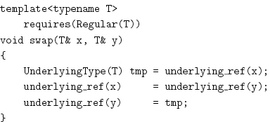
which could also be accomplished with:

   swap_basic(underlying_ref(x), underlying_ref(y));

Many rearrangement algorithms can be modified for use with underlying type simply by reimplementing exchange_values and cycle_from the same way we reimplemented swap.

To handle other rearrangement algorithms, we use an iterator adapter. Such an adapter has the same traversal operations as the original iterator, but the value type is replaced by the underlying type of the original value type; source returns underlying_ref(source(x.i)), and sink returns underlying_ref(sink(x.i)), where x is the adapter object, and i is the original iterator object inside x.

Exercise 12.9 Implement such an adapter that works for all iterator concepts.

Now we can reimplement reverse_n_with_temporary_buffer as follows:

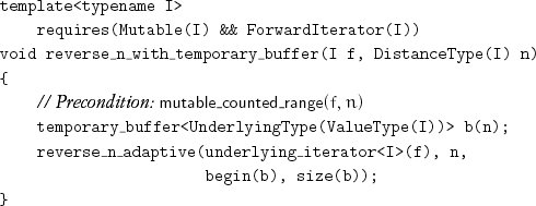
where underlying_iterator is the adapter from Exercise 12.9.

Project 12.5 Use underlying type systematically throughout a major C++ library, such as STL, or design a new library based on the ideas in this book.

12.4 Conclusions

We extended the structure types and constant-size array types of C++ to dynamic data structures with remote parts. The concepts of ownership and regularity determine treatment of parts by copy construction, assignment, equality, and total ordering. As we showed for the case of dynamic sequences, useful varieties of data structures should be carefully implemented, classified, and documented so that programmers can select the best one for each application. Rearrangements on nested data structures are efficiently implemented by temporarily relaxing the ownership invariant.