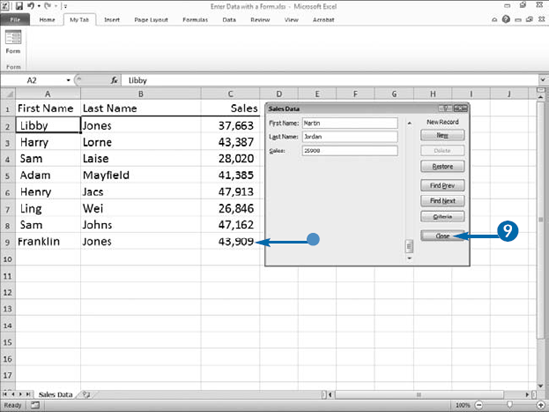
People often organize data into lists. You can use Excel to manage lists. In Excel, a list is a rectangular section of a worksheet structured as a set of columns and rows. You call each column a field and you give each field a label. Field labels appear on the first row of a list. Each row in a list is called a record. For example, you can have a list of sales people organized as follows: First Name, Last Name, Sales. You label the first column First Name, you label the second column Last Name, and you label the last column Sales. On each row of your list, in the First Name field, first names appear; in the Last Name field, last names appear; and in the Sales field, sales appear.
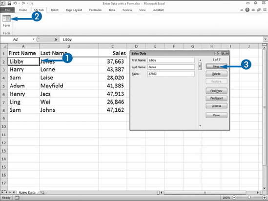
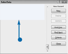
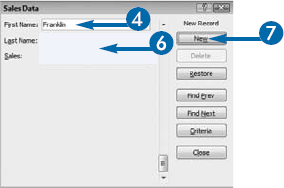
In Excel, you can use a form to simplify entering data into a list. A form speeds up your data entry by providing a blank field for each column in your list. A form uses field labels as field names. You can type your data into the form and use the Tab key to move from field to field. After you complete each set of fields, click the Next button to enter the record into a row in your list and then type in a new record. You can use the Find Prev (Previous) and Find Next buttons to move backward and forward through your list to view or modify your data.
You must add the Form button to the Ribbon or the Quick Access Toolbar before you can use forms. Refer to Chapter 17 to learn how to add items to the Ribbon and the Quick Access Toolbar.
You can sort a list so that you can easily find and group data. You can use the Sort buttons on the Data tab to sort. When you sort, you rearrange your data in ascending or descending order. The meaning of these terms depends on the kind of data you are sorting. Dates sorted in ascending order show the earliest date first. Dates sorted in descending order show the latest date first. Text sorted in ascending order sorts A to Z. Text sorted in descending order sorts Z to A. Numeric data sorted in ascending order sorts from the lowest number to the highest. Numeric data sorted in descending order sorts from the highest number to the lowest.
With filtering, you can display only the data that you want to display. For example, if you have a list that includes data for four quarters, you can choose to view data for the first quarter only.
When you click Filter on the Data tab, Excel places AutoFilter buttons next to each of the fields in your list. You can use the AutoFilter buttons to display a menu with options that enable you to sort and filter your data. You can click a sort option to sort a column or you can filter by deselecting the items that you do not want to appear in your list. You can apply filters to multiple columns in the same list. Each filter you apply narrows your selection further.
If after applying a sort or filter you make changes to your data, you can refresh you data by clicking Reapply.
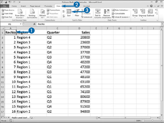
Perform Simple Sorts and Filters
Sort a List


Click A to Z to sort from lowest to highest — ascending order.
Click Z to A to sort from highest to lowest — descending order.
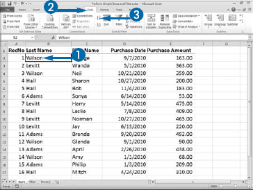
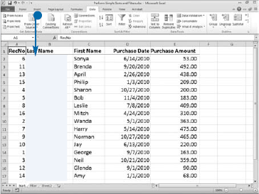
Excel sorts your list by the column you selected.
Extra
When you perform a filter, Excel places AutoFilter buttons (
To clear all filters, click Clear in the Sort & Filter group on the Data tab. To remove the AutoFilter buttons next to your field names, click Filter. To bring the AutoFilter buttons back, click Filter again. Filter toggles the Sort & Filter feature on and off.
Excel defines different sorts as follows: For numbers, ascending order goes from the smallest number to the largest. For text that includes numerals, as in U2 and K12, ascending order places numerals before symbols and symbols before letters. Case does not matter unless you click Options in the Sort dialog box and then click the Case Sensitive check box (
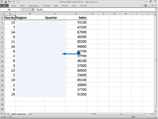
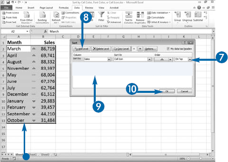
When you perform a simple sort, you can only sort by one column in your list. If you need to sort multiple columns, you must perform a multilevel sort. With a multilevel sort, you can, for example, sort by quarter and within a quarter by region.
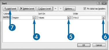
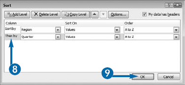
To perform a multilevel sort, you use the Sort dialog box. If your list has column labels, make sure the My data has headers check box is selected. You will select the first sort level, add a level, and then select the next sort level. For example, if you are sorting by quarter and then within quarter by region, the Quarter field is your first sort level and the Region field is your second sort level. You can have up to 64 sort levels.
In the Sort dialog box, use the Column drop-down list to choose the column you want to sort. Use the Sort On drop-down list to choose what you want to base your sort on. If you want to sort on text, dates, or numbers, choose Values. Use the Order drop-down list to choose a sort order. If you want to sort in ascending order, choose A to Z. If you want to sort in descending order, choose Z to A.
If you choose ascending order, Excel sorts values in the following order: numbers, text, logical values, error values blanks. If you choose descending order, Excel reverses that order for everything except blanks, which are sorted last. You can also sort by cell color, font color, or cell icon. See the section "Sort by Cell Color, Font Color, or Cell Icon" to learn more.
Extra
If you are sorting a list, click in any cell in the list and Excel will select the entire list when you open the Sort dialog box. If you are sorting a range of cells that are not a list, select the cells and then click Sort on the Data tab to open the Sort dialog box. If necessary, Deselect the My data has headers check box.
In the Sort dialog box, click the Delete Level button to delete a level of sort. Click the Copy Level button to copy a level of sort. Click (
By default, Excel sorts from top to bottom. If you want to sort from left to right, click Sort on the Data tab. The Sort dialog box appears. Click the Options button. The Sort Options dialog box appears. Click Sort Left to Right (
By default, sorts are not case-sensitive. If you want to make them case-sensitive, click Case Sensitive (
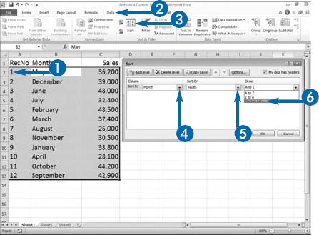
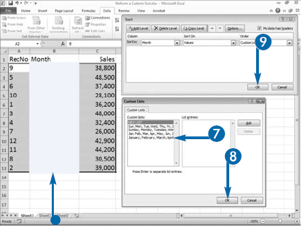
You can use a custom sort to sort in an order other than ascending or descending. For example, if you have a list of sales data and you want to sort it by the months in a year — January through December — you can use a custom sort.
When you choose Custom List in the Order drop-down list in the Sort dialog box, the Custom Lists dialog box appears. There you can choose a custom sort order such as days of the week or months of the year. You can also add your own list to the Custom Lists dialog box and use it to sort. For example, if you often order your data North, South, East, West, you can add that list to the Custom Lists dialog box and use it to sort.
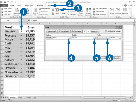
You can use conditional formatting to format your data. You can format your data with cell colors, font colors, or cell icons. You can then use the Sort dialog box to sort data based on the cell color, font color, or cell icon. For example, you can use an icon to mark the top one-third, the second one-third, and the lowest one-third of sales figures. You can then sort your data based on the icon assigned. You can also manually assign cells font and cell colors and then sort by the colors. Each level determines where the cell color, font color, or cell icon appears, either at the top of the list or at the bottom of the list.
You will find that there are times when you are not interested in all the data in your list. For example, you have a list of employee salaries but you only want to examine the salaries of people who earn between $50,000 and $100,000 per year. Excel's AutoFilter feature can aid you. By filtering, you can find every value in your list that falls between two values, equals a value, is greater than a value, or meets a number of other criteria you specify. Filtering hides data. When you remove the filter, Excel brings the data back.
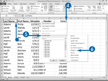
When you click the Filter button on the Data tab, AutoFilter buttons appear to the right of every column label. You can click a column's AutoFilter button and then select Date Filters for date fields, Text Filters for text fields, and Number Filters for numeric fields. When you select one of these options, a menu appears. From this menu, you can select the criteria you want to apply, such as between two values.
You can apply multiple filters. By applying multiple filters, you can quickly narrow a long list to the few records of interest to you. For example, if you want to examine the salaries of women who earn between $50,000 and $100,000 per year, you can filter your salary column for salaries between $50,000 and $100,000 and then filter your gender column for F (females).
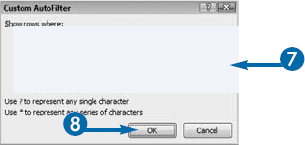
In addition to choosing a filter type from the filter menu, you can choose to create a custom filter. By using a custom AutoFilter, you can create multiple filters in a single column by using the And or Or filter.
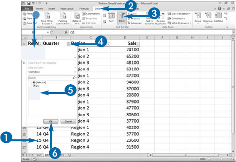
Perform Complex Filters
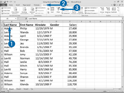
AutoFilter buttons appear next to all your column labels.


Alternatively, click Text Filters if you chose a text field or Date Filters if you chose a date field.
A menu appears.


Excel filters the list.
You can filter additional columns.
Click the Data tab and then click Clear in the Sort & Filter group to clear your filter.
Once you have created a list of data, you may want to retrieve specific information. Using Excel's Advanced Filter, you can set up complex filters and use them to limit the data you retrieve.
When using Excel's Advanced Filter, you must identify an area called the criteria range. In the criteria range, you tell Excel exactly what you are looking for. For example, you can tell Excel you want to retrieve all people with an income of $100,000 or more.
With advanced filtering, you can go beyond the limitations of the AutoFilter command. You can use advanced filtering to create two or more filters and easily coordinate a set of filters among columns. For example, you can filter a list to find all females with an income more than $100,000 and all males with an income less than $100,000.
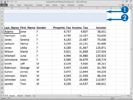
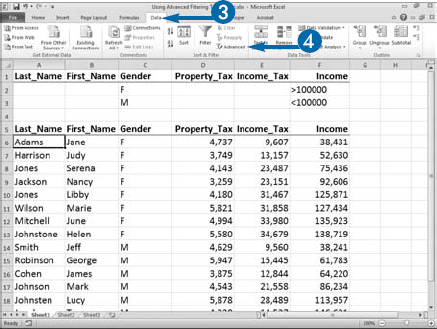
Advanced filtering requires a bit of work, even when you are using the Advanced Filter menu command. You must find a block of cells on your worksheet and create a criteria range. Use one or more column heads from a list. In the cell below each label, type the criteria by which to filter each column, such as >100000 to find people with an income greater than $100,000 and M to find all males. See the previous section, "Enter Criteria to Find Records," for detailed instructions.
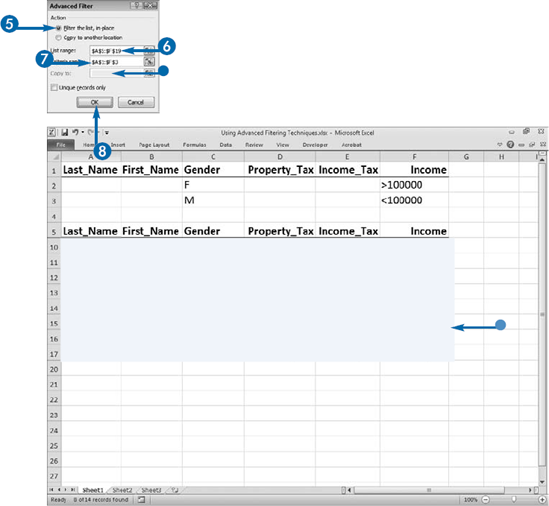
You have two options when you create any type of filtered list. You can have your filtered list appear in place — under the column heads of your unfiltered list — thereby hiding the unfiltered list. Or, you can have your filtered list appear in another location, thereby enabling you to keep your original list in your worksheet. If you want to filter your list in place, in the Advanced Filter dialog box, click Filter the list, in-place. If you want to keep your unfiltered list in your worksheet, in the Advanced Filter dialog box, click Copy to another location and then enter the location where you want to place your filtered list in the Copy to field.
Make sure your Copy to range has enough room below it to include all the values that may return in the filtered list. If you place the Copy to range above your original list, the results may overwrite the list and disrupt the filtering. Placing the copy to the side of the list or on another worksheet protects your original list.
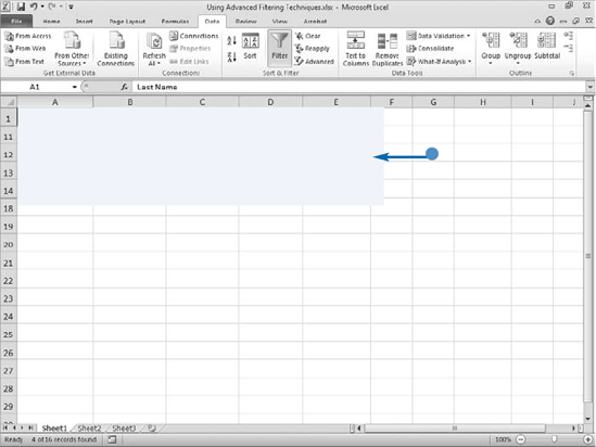
Using Advanced Filtering Techniques
You can click Copy to another location to copy the list to another location and retain the original list.
If you chose to copy the filtered list in Step 5, enter the first cell in the range where you want to place the copy.
The filtered list appears.
Click Clear on the Data tab in the Sort & Filter group to clear your filter.
Apply It
By default, the criteria you enter are not case-sensitive. Excel considers "JONES" the same as "jones". You can, however, use the EXACT function to create criteria that are case-sensitive. To start, create a column label in your criteria range and name it Exact Match. In the field below the Exact Match column label, type the EXACT function. For example, type =EXACT(A10,"Jones"). A10 refers to the column you want to filter, A, and the first row under the label of the list range, 10.
Now, click the Data tab. Click Advanced in the Sort & Filter group. The Advanced Filter dialog box appears. Click the Filter the list, in-place or Copy to another location radio button (
If you name your list range Database, your criteria range Criteria, and your Copy to range"Extract, Excel automatically places these values into the Advanced Filter dialog box.
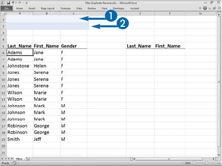
Excel provides many tools for managing long lists. With such lists, you may need to identify and display unique records. You might, for example, want to have a unique list of your female customers.
Excel provides tools for displaying unique records that meet your criteria. You start with a worksheet formatted as a list, in which some of the records are duplicates, meaning the values in two or more rows are the same. Then use Excel's advanced filtering tool to identify and filter the duplicates. You must specify the criteria by which you want to filter your data. Your criteria consist of a least two rows, one with one or more labels and the other with criteria. See the section, "Enter Criteria to Find Records" for detailed information on how to set up your criteria. Because Excel hides the duplicate rows, the best placement for your criteria is above your list or on another worksheet. Place at least one blank row between your criteria range and your list.
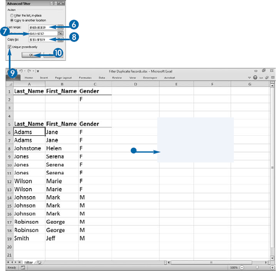
You have two options when you create a filtered list using Excel's advanced filtering tool. You can have your filtered list appear in place — under the column heads of your unfiltered list — thereby temporarily replacing your unfiltered list, or you can place your filtered list in another location. Use the Copy to field in the Advanced Filter dialog box to specify the location. If you copy your list to another location, you can specify which fields you want to copy by typing the column labels into the area you specify in the Copy to field.
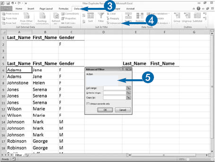
Filter Duplicate Records
The Advanced Filter dialog box appears.


The filtered list appears.
Click Clear on the Data tab in the Sort & Filter group to clear your filter.
Apply It
You can use Excel's advanced filtering feature to display a unique list — a list with just one copy of rows in which every field in every column is the same. Click the Data tab. Click Advanced in the Sort & Filter group. The Advanced Filter dialog box appears. Select whether you want to filter your list in place or to another location (
Filtering duplicate records temporarily removes them from view. If you want to delete duplicate records permanently, select your list, and click the Data tab. Then in the Data tools group, click Remove Duplicates. The Remove Duplicates dialog box appears. If your list has headers, click My data has headers (
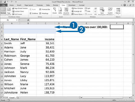
Like standard worksheet functions, database functions enable you to perform calculations and summarize data patterns. Database functions are meant for lists and are especially good at summarizing the subsets you create by filtering your list. Most database functions combine two tasks: they filter a group of records based on values in a single column, and then they count the records or perform another simple operation on the filtered data.
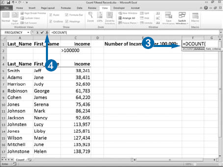
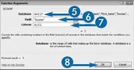
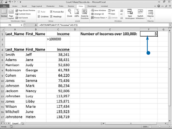
DCOUNT is a database function that counts the number of cells containing numbers. DCOUNT takes three arguments. The first argument, Database, identifies the cell range for the entire list. The second argument, Field, identifies the column you want to count. You can enter the column label enclosed in quotes; for example, "Income", or you can enter the column number. The first column in the list is 1, the second is 2, and so on. In the third argument, Criteria, you provide Excel with the range location of your criteria for extracting information. For example, your criteria could be Income >100000, where Income is the column label. You build the criteria manually, copying column labels and defining the conditions in the cells below them. You then place the range in your formula. You can use any range as long as the range includes at least one column label and one cell below it. If you want to count every record in the list, leave the cells in your criteria range below your label blank. If your criteria is text, enter it in the format = "= Text Value". If you do not, Excel may calculate improperly.
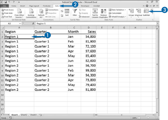
After you sort, you can group your data into categories, such as quarter and region, and you can perform calculations so that you can compare one category with another. If you have a sort defined for at least one column, you can find the average, sum, min, max, number of items, and more for that column or another column. Excel calls this feature subtotaling.
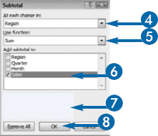
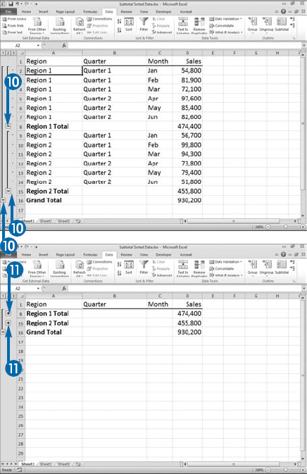
When you apply the subtotaling feature to a list, Excel outlines the data. You can expand and collapse the outline to see different views of the data. For example, if you subtotal by region, you can collapse the data so that you only see regional and grand totals. Your subtotals and grand totals can appear either above or below each category. If you want them to appear below the category, select Summary below data. You can choose to enter a page break after each subtotal. This feature places each category on a separate page when you print.
You can create several levels of subtotals for a single sorted list. You start by using the Subtotal dialog box to create the highest-level subtotal. Then you open the Subtotal dialog box again to create the next-level subtotal. You can create up to eight levels. Make sure you have not checked the Replace current subtotals check box in the Subtotal dialog box as you create each level.
You can create subtotals on columns other than the one defining the sort. For example, if you sort by quarter, you can subtotal sales. You can also do a count on a column with text entries. To remove subtotals, click the Remove All button in the Subtotal dialog box.
Apply It
You can manually group the rows and columns in your worksheet. For example, you can hide the details related to daily sales so that you can compare monthly sales. Select the columns or rows you want to group. Click the Data tab. Click Group in the Outline group. A menu appears. Click Group. The Group dialog box appears. Click a radio button option to select either the Columns or Rows option. Click Rows if you want to group rows (
To remove a group, click the Data tab. Click Ungroup in the Outline group. A menu appears. Click Ungroup. The Ungroup dialog box appears. Click a radio button option to select either Columns or Rows. Click Columns if you want to ungroup columns. Click Rows if you want to Ungroup rows. Click OK.
When you outline a worksheet, Excel places buttons above the worksheet column labels and to the left of the worksheet row labels. You can use these buttons to collapse and expand areas of your worksheet. The collapse buttons appear as minus signs (–). The expand buttons appear as plus signs (+). When you click a minus sign, Excel hides columns or rows. When you click a plus sign, Excel reveals columns or rows.
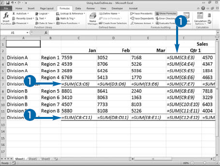
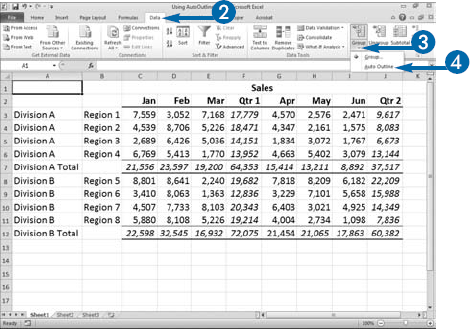
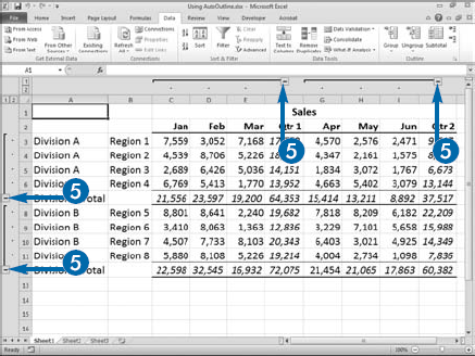
Excel can automatically outline your worksheet for you. For example, if you have a worksheet with sales data in columns for January, February, and March and a formula that calculates quarterly totals by summing January, February, and March and then does the same for April, May, and June, you can outline your columns by quarter. If on that same worksheet, you have data on rows for two divisions, Division A and Division B, and you have formulas that calculate totals by division, you can outline your rows by division.
The Auto Outline feature uses formulas to determine where to place expand and collapse buttons. Expand and collapse buttons appear on columns with formulas. So, to create an outline, enter formulas where you want the collapsible buttons to appear. If, for example, you want to collapse your worksheet so that you only see quarterly summaries and division totals, enter formulas to calculate the quarterly summaries and the division totals.
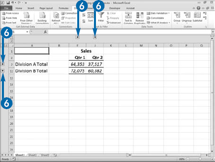
The Auto Outline feature gives you a great deal of flexibility. You can expand or collapse each area individually. For example, you can collapse Quarter 1 so that you only see the summary, while leaving the details of Quarter 2 available for viewing.
Apply It
To remove an Auto Outline, click the Data tab. Click the down arrow under Ungroup in the Outline group. A menu appears. Click Clear Outline.
If you want to outline a range of cells instead of an entire worksheet, select the range you want to outline. Click the Data tab. Click the down arrow under Group. A menu appears. Click Auto Outline. Excel outlines the range. You can now use the Expand (
You can have Excel automatically apply a style each time you create an outline. Click the Data tab. Click the launcher in the Outline group. The Settings dialog box appears. Click Automatic Styles. Click OK. Now when you create an outline, Excel automatically applies a style. If you want to apply a style to an Auto Outline manually, select the range. Click the Data tab. Click the launcher in the Outline group. The Settings dialog box appears. Click Apply Styles. Excel applies the style.
You can use the Expand and Collapse buttons on the Ribbon to expand and collapse your outline. Select the area you want to expand or collapse and then click the Expand button (
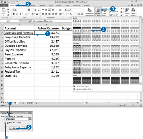
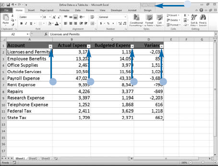
In Excel, a table is a special type of list. Like all lists, a table is a set of columns and rows where each column represents a single type of data. To create a table, you simply define a list as a table. When you define a list as a table, Excel adds AutoFilter buttons to each column label, enabling you to readily sort and filter your data. To learn how to use these AutoFilter buttons, see section, "Perform Simple Sorts and Filters."
Tables have a unique quality. When you enter a formula into a table column that does not have any data in it, it"becomes a calculated column. Calculated columns automatically calculate when you create a new row. However, if you type a formula in a table column that already contains data, Excel does not automatically create a calculated column. You, however, can turn the column into a calculated column by clicking the Create Calculated Column button that appears after you type the formula.
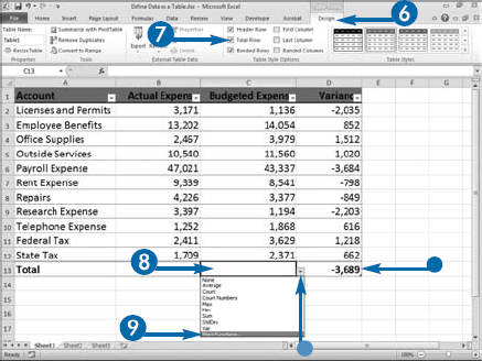
By selecting Total Row on the Design tab, you can easily add totals to your Excel table. Totals enable you to find the sum, count, max, min, or other value based on a column. You can calculate a different value for each column in your table.
You can create a new table row by pressing the Tab key while in the last field in the last row of your table. To create a new table column, type the label name next to the last label in the last column of the table.
Extra
If you want to add a formula to your table but you do not want it to be a calculated column, click Undo Calculated Column on the AutoCorrect Options menu that automatically appears when you complete the entry of your formula.
If you do not want Excel to create calculated fields automatically, click the File tab. A menu appears. Click Options. Click Proofing. Click the AutoCorrect Options button. The AutoCorrect dialog box appears. Click the AutoFormat As You Type tab. Deselect Fill formulas in tables to create calculated columns (
You can use the Insert and Delete options on the Home tab in the Cells group to insert and delete rows and columns in your table. To insert rows or columns, click anywhere in your table. Click the Home tab. Click the down arrow next to Insert in the Cells group and then click Insert Table Rows Above or Insert Table Columns to Left.
To delete rows or columns, click anywhere in your table. Click the Home tab. Click the down arrow next to Delete in the Cells group and then click Delete Table Rows or Delete Table Columns.
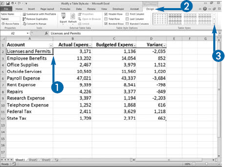
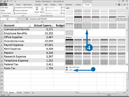
Table styles format the rows and columns of your table to make your table easier to read. When you create a table, you apply a style. You can use the style gallery to change or remove a style. The style gallery provides a large number of styles from which to choose. As you move your mouse pointer over each style in the gallery, Excel gives you a live preview of how that style will appear when you apply it. You can use the Clear"button at the bottom of the Style gallery to remove a style.
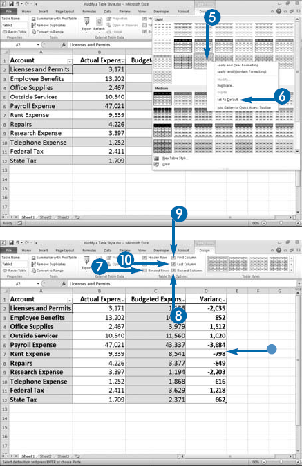
Excel also provides a number of table-style options you can use to modify a table style. By choosing banded rows or banded columns, you can have every other row or every other column appear in a different color. You can also apply special formatting to the last column or the first column in your table if you want the titles, totals, or"whatever information you have in those columns to stand out.
Table styles make your table more attractive and user friendly. If you have a favorite style, you can set that style to be the default. Then, whenever you define a list to be a table, Excel will apply that style.
If you do not want your data formatted as a table, you can change a table back to a regular range of cells. If you need to add columns or rows to your table, you can make your table larger. And, if you do not see a table style you like in the gallery, you can modify an existing style and create a new style.
Modify a Table Style
A gallery of styles appears.
Click Clear to remove a style from your table.
A menu appears.
Excel makes the style the default style.
Excel reformats the table.
Apply It
You can convert a table back to a regular range of cells. Click anywhere in your table, click the Design tab, and then click Convert to Range in the Tools group. At the prompt, click Yes. Excel converts the table to a normal range and removes the AutoFilter buttons.
You can easily add columns your table. Click any cell in your table. The Table tools appear. Click the Design tab and then click Resize Table in the Properties group. The Resize Table dialog box appears. Enter a new range in the Select the New Data Range for Your Table field and then click OK.
You can create your own table style by modifying an existing style. Click in your table. Click the Design tab. Click the More button (
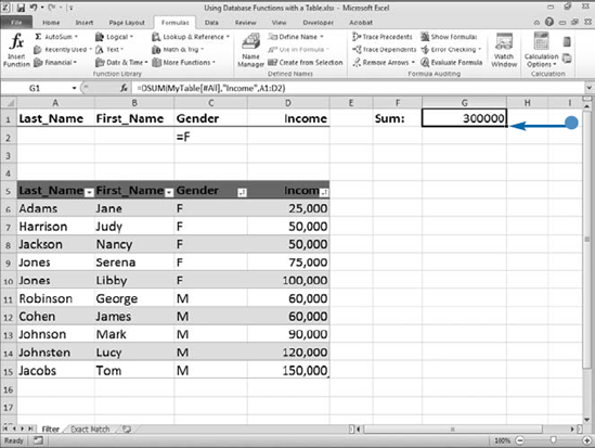
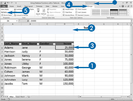
Database functions were designed to be used with lists. A table is a type of list. Using database functions with a table provides advantages because every table has a name and Excel will use the table's name in the database function. Because the function is referencing a table name, the table can grow to an unlimited number of rows and the reference will still be valid. In fact, no matter how many records you add or delete, your table reference remains valid.
DSUM is a database function that totals the numbers of cells in a column that match the criteria you enter. DSUM takes three arguments. The first argument, Database, is the table range. The second argument, Field, identifies the the column you want to sum. You can enter the column label enclosed in quotes; for example, "Income" or you can enter the column number. The first column in the table is 1, the second is 2, and so on. In the third argument, Criteria, you provide Excel with the range location of your criteria. For example, your criteria could be Gender = "=F", where Gender is the column label. You build the criteria manually, copying column labels and defining the conditions in the cells below them. You then place the range in your formula. You can use any range as long as the range includes at least one column label and one cell below it. If you want to add every record in the list, leave the cells in your criteria range below your labels blank. If your criteria is text, enter it in the format = "= Text Value".
Using Database Functions with a Table
The Table tools appear.
Alternatively, click the function on the AutoComplete list.
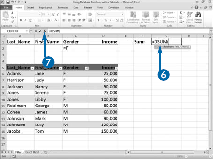
Excel enters the table name.
Or type the column's number or the column's range.

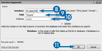
Excel calculates the result.
Click Clear on the Data tab in the Sort & Filter group to clear your filter.