
1.3 Fundamentals of Digital Signal Processing
The fundamentals of digital signal processing consist of the description of digital signals—in the context of this book we use digital audio signals—as a sequence of numbers with appropriate number representation and the description of digital systems, which are described by software algorithms to calculate an output sequence of numbers from an input sequence of numbers. The visual representation of digital systems is achieved by functional block diagram representations or signal flow graphs. We will focus on some simple basics as an introduction to the notation and refer the reader to the literature for an introduction to digital signal processing [ME93, Orf96, Zöl05, MSY98, Mit01].
1.3.1 Digital Signals
The digital signal representation of an analog audio signal as a sequence of numbers is achieved by an analog-to-digital converter (ADC). The ADC performs sampling of the amplitudes of the analog signal x(t) on an equidistant grid along the horizontal time axis and quantization of the amplitudes to fixed samples represented by numbers x(n) along the vertical amplitude axis (see Fig. 1.11). The samples are shown as vertical lines with dots on the top. The analog signal x(t) denotes the signal amplitude over continuous time t in micro seconds. Following the ADC, the digital (discrete time and quantized amplitude) signal is a sequence (stream) of samples x(n) represented by numbers over the discrete time index n. The time distance between two consecutive samples is termed sampling interval T (sampling period) and the reciprocal is the sampling frequency fS = 1/T (sampling rate). The sampling frequency reflects the number of samples per second in Hertz (Hz). According to the sampling theorem, it has to be chosen as twice the highest frequency fmax (signal bandwidth) contained in the analog signal, namely fS > 2 · fmax. If we are forced to use a fixed sampling frequency fS, we have to make sure that our input signal to be sampled has a bandwidth according to fmax = fS /2. If not, we have to reject higher frequencies by filtering with a lowpass filter which only passes all frequencies up to fmax. The digital signal is then passed to a DAFX box (digital system), which in this example performs a simple multiplication of each sample by 0.5 to deliver the output signal y(n) = 0.5 · x(n). This signal y(n) is then forwarded to a digital-to-analog converter DAC, which reconstructs the analog signal y(t). The output signal y(t) has half the amplitude of the input signal x(t).
Figure 1.11 Sampling and quantizing by ADC, digital audio effects and reconstruction by DAC.
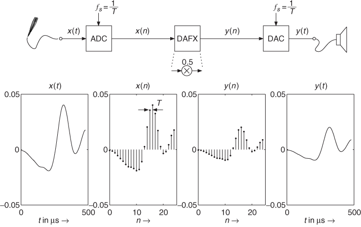
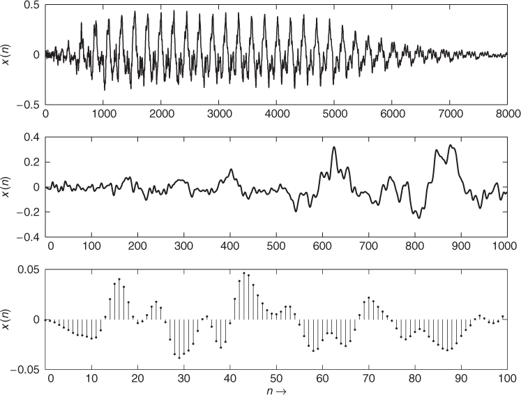
Figure 1.12 shows some digital signals to demonstrate different graphical representations (see M-file 1.1). The upper part shows 8000 samples, the middle part the first 1000 samples and the lower part shows the first 100 samples out of a digital audio signal. Only if the number of samples inside a figure is sufficiently low, will the line with dot graphical representation be used for a digital signal.
M-file 1.1 (figure1_03.m)
% Author: U. Zölzer
[x,FS,NBITS]=wavread(’ton2.wav’);
figure(1)
subplot(3,1,1);
plot(0:7999,x(1:8000));ylabel(’x(n)’);
subplot(3,1,2);
plot(0:999,x(1:1000));ylabel(’x(n)’);
subplot(3,1,3);
stem(0:99,x(1:100),’.’);ylabel(’x(n)’);
xlabel(’n ightarrow’);
Figure 1.12 Different time representations for digital audio signals.
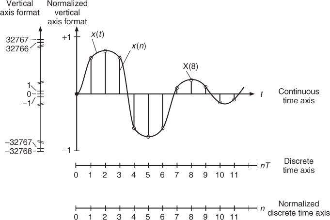
Two different vertical scale formats for digital audio signals are shown in Figure 1.13. The quantization of the amplitudes to fixed numbers in the range −32768 … 32767 is based on a 16-bit representation of the sample amplitudes which allows 216 quantized values in the range −215 … 215 − 1. For a general w-bit representation the number range is −2w−1 … 2w−1 − 1. This representation is called the integer number representation. If we divide all integer numbers by the maximum absolute value, for example 32768, we come to the normalized vertical scale in Figure 1.13, which is in the range −1 … 1 − Q, where Q is the quantization step size. It and can be calculated by Q = 2−(w−1), which leads to Q = 3.0518 × 10⁻⁵ for w = 16. Figure 1.13 also displays the horizontal scale formats, namely the continuous-time axis, the discrete-time axis and the normalized discrete-time axis, which will be used normally. After this narrow description we can define a digital signal as a discrete-time and discrete-amplitude signal, which is formed by sampling an analog signal and by quantization of the amplitude onto a fixed number of amplitude values. The digital signal is represented by a sequence of numbers x(n). Reconstruction of analog signals can be performed by DACs. Further details of ADCs and DACs and the related theory can be found in the literature. For our discussion of digital audio effects this short introduction to digital signals is sufficient.
Figure 1.13 Vertical and horizontal scale formats for digital audio signals.
Signal processing algorithms usually process signals by either block processing or sample-by-sample processing. Examples for digital audio effects are presented in [Arf98]. For block processing, samples are first collected in a memory buffer and then processed each time the buffer is completely filled with new data. Examples of such algorithms are fast Fourier transforms (FFTs) for spectra computations and fast convolution. In sample processing algorithms, each input sample is processed on a sample-by-sample basis.
A basic algorithm for weighting of a sound x(n) (see Figure 1.11) by a constant factor a demonstrates a sample-by-sample processing (see M-file 1.2). The input signal is represented by a vector of numbers [x(1), x(2),…, x(length(x))].
M-file 1.2 (sbs_alg.m)
% Author: U. Zölzer
% Read input sound file into vector x(n) and sampling frequency FS
[x,FS]=wavread(’input filename’);
% Sample-by sample algorithm y(n)=a*x(n)
for n=1:length(x),
y(n)=a * x(n);
end;
% Write y(n) into output sound file with number of
% bits Nbits and sampling frequency FS
wavwrite(y,FS,Nbits,’output filename’);
1.3.2 Spectrum Analysis of Digital Signals
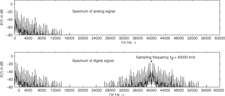
The spectrum of a signal shows the distribution of energy over the frequency range. The upper part of Figure 1.14 shows the spectrum of a short time slot of an analog audio signal. The frequencies range up to 20 kHz. The sampling and quantization of the analog signal with sampling frequency of fS = 40 kHz leads to a corresponding digital signal. The spectrum of the digital signal of the same time slot is shown in the lower part of Figure 1.14. The sampling operation leads to a replication of the baseband spectrum of the analog signal [Orf96]. The frequency contents from 0 Hz up to 20 kHz of the analog signal now also appear from 40 kHz up to 60 kHz and the folded version of it from 40 kHz down to 20 kHz. The replication of this first image of the baseband spectrum at 40 kHz will now also appear at integer multiples of the sampling frequency of fS = 40 kHz. But notice that the spectrum of the digital signal from 0 up to 20 kHz shows exactly the same shape as the spectrum of the analog signal. The reconstruction of the analog signal out of the digital signal is achieved by simply lowpass filtering the digital signal, rejecting frequencies higher than fS /2 = 20 kHz. If we consider the spectrum of the digital signal in the lower part of Fig. 1.14 and reject all frequencies higher than 20 kHz, we come back to the spectrum of the analog signal in the upper part of the figure.
Figure 1.14 Spectra of analog and digital signals.
Discrete Fourier Transform
The spectrum of a digital signal can be computed by the discrete Fourier transform (DFT) which is given by
1.1 
The fast version of the above formula is called the fast Fourier transform (FFT). The FFT takes N consecutive samples out of the signal x(n) and performs a mathematical operation to yield N samples X(k) of the spectrum of the signal. Figure 1.15 demonstrates the results of a 16-point FFT applied to 16 samples of a cosine signal. The result is normalized by N according to X=abs(fft(x,N))/N;.
Figure 1.15 Spectrum analysis with FFT algorithm: (a) digital cosine with N = 16 samples, (b) magnitude spectrum |X(k)| with N = 16 frequency samples and (c) magnitude spectrum |X(f)| from 0 Hz up to the sampling frequency fS = 40 000 Hz.
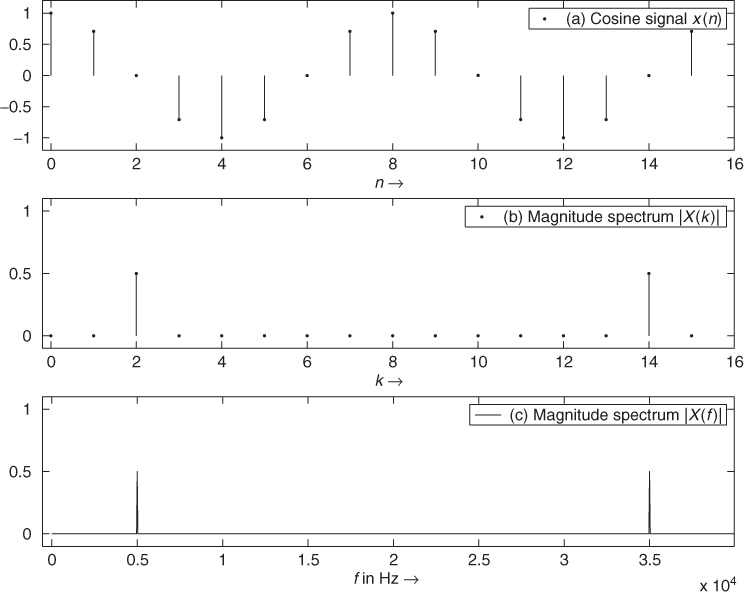
The N samples X(k) = XR(k) + jXI(k) are complex-valued with a real part XR(k) and an imaginary part XI(k) from which one can compute the absolute value
1.2 ![]()
which is the magnitude spectrum, and the phase
1.3 ![]()
which is the phase spectrum. Figure 1.15 also shows that the FFT algorithm leads to N equidistant frequency points which give N samples of the spectrum of the signal starting from 0 Hz in steps of ![]() up to
up to ![]() . These frequency points are given by
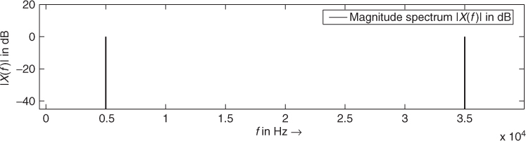
. These frequency points are given by ![]() , where k is running from 0, 1, 2, …, N − 1. The magnitude spectrum |X(f)| is often plotted over a logarithmic amplitude scale according to
, where k is running from 0, 1, 2, …, N − 1. The magnitude spectrum |X(f)| is often plotted over a logarithmic amplitude scale according to ![]() which gives 0 dB for a sinusoid of maximum amplitude ±1. This normalization is equivalent to
which gives 0 dB for a sinusoid of maximum amplitude ±1. This normalization is equivalent to ![]() . Figure 1.16 shows this representation of the example from Fig. 1.15. Images of the baseband spectrum occur at the sampling frequency fS and multiples of fS. Therefore we see the original frequency at 5 kHz and in the first image spectrum the folded frequency fS − fcosine = 40 000 Hz − 5000 Hz = 35 000 Hz.
. Figure 1.16 shows this representation of the example from Fig. 1.15. Images of the baseband spectrum occur at the sampling frequency fS and multiples of fS. Therefore we see the original frequency at 5 kHz and in the first image spectrum the folded frequency fS − fcosine = 40 000 Hz − 5000 Hz = 35 000 Hz.
Figure 1.16 Magnitude spectrum |X(f)| in dB from 0 Hz up to the sampling frequency fS = 40000 Hz.
Inverse Discrete Fourier Transform (IDFT)
Whilst the DFT is used as the transform from the discrete-time domain to the discrete-frequency domain for spectrum analysis, the inverse discrete Fourier transform (IDFT) allows the transform from the discrete-frequency domain to the discrete-time domain. The IDFT algorithm is given by
1.4 
The fast version of the IDFT is called the inverse Fast Fourier transform (IFFT). Taking N complex-valued numbers with the property X(k) = X*(N − k) in the frequency domain and then performing the IFFT gives N discrete-time samples x(n), which are real-valued.
Frequency Resolution: Zero-padding and Window Functions
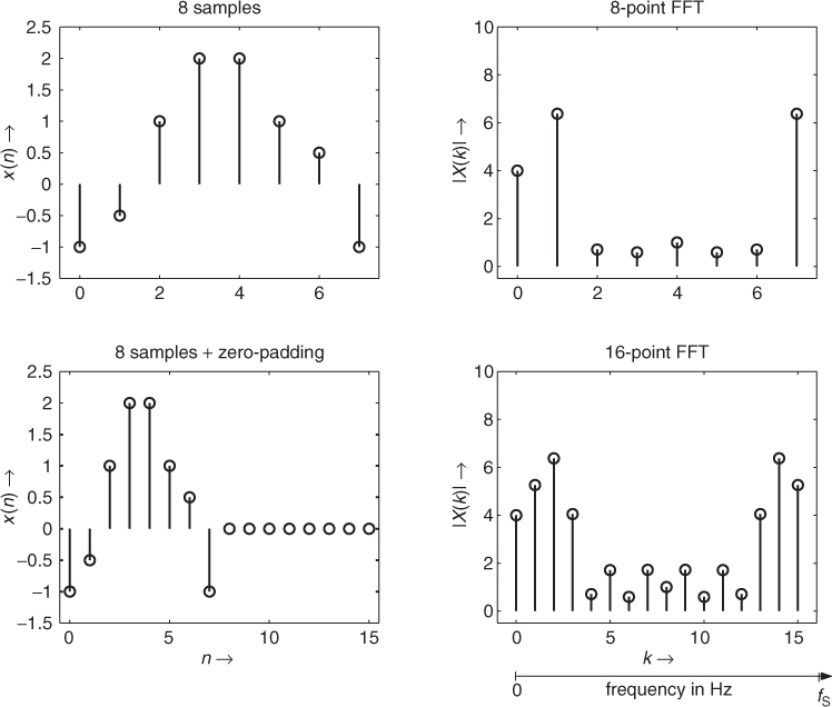
To increase the frequency resolution for spectrum analysis we simply take more samples for the FFT algorithm. Typical numbers for the FFT resolution are N = 256, 512, 1024, 2048, 4096 and 8192. If we are only interested in computing the spectrum of 64 samples and would like to increase the frequency resolution from fS/64 to fS/1024, we have to extend the sequence of 64 audio samples by adding zero samples up to the length 1024 and then perform an 1024-point FFT. This technique is called zero-padding and is illustrated in Figure 1.17 and by M-file 1.3. The upper left part shows the original sequence of eight samples and the upper right part shows the corresponding eight-point FFT result. The lower left part illustrates the adding of eight zero samples to the original eight-sample sequence up to the length N = 16. The lower right part illustrates the magnitude spectrum |X(k)| resulting from the 16-point FFT of the zero-padded sequence of length N = 16. Notice the increase in frequency resolution between the eight-point and 16-point FFT. Between each frequency bin of the upper spectrum a new frequency bin in the lower spectrum is calculated. Bins k = 0, 2, 4, 6, 8, 10, 12, 14 of the 16-point FFT correspond to bins k = 0, 1, 2, 3, 4, 5, 6, 7 of the eight-point FFT. These N frequency bins cover the frequency range from 0 Hz up to ![]() .
.
Figure 1.17 Zero-padding to increase frequency resolution.
M-file 1.3 (figure1_17.m)
%Author: U. Zölzer
x1=[-1 -0.5 1 2 2 1 0.5 -1];
x2(16)=0;
x2(1:8)=x1;
subplot(221);
stem(0:1:7,x1);axis([-0.5 7.5 -1.5 2.5]);
ylabel(’x(n) ightarrow’);title(’8 samples'),
subplot(222);
stem(0:1:7,abs(fft(x1)));axis([-0.5 7.5 -0.5 10]);
ylabel(’|X(k)| ightarrow’);title(’8-point FFT’);
subplot(223);
stem(0:1:15,x2);axis([-0.5 15.5 -1.5 2.5]);
xlabel(’n ightarrow’);ylabel(’x(n) ightarrow’);
title(’8 samples+zero-padding’);
subplot(224);
stem(0:1:15,abs(fft(x2)));axis([-1 16 -0.5 10]);
xlabel(’k ightarrow’);ylabel(’|X(k)| ightarrow’);
title(’16-point FFT’);
The leakage effect occurs due to cutting out N samples from the signal. This effect is shown in the upper part of Figure 1.18 and demonstrated by the corresponding M-file 1.4. The cosine spectrum is smeared around the frequency. We can reduce the leakage effect by selecting a window function like Blackman window and Hamming window
1.5 ![]()
1.6 ![]()
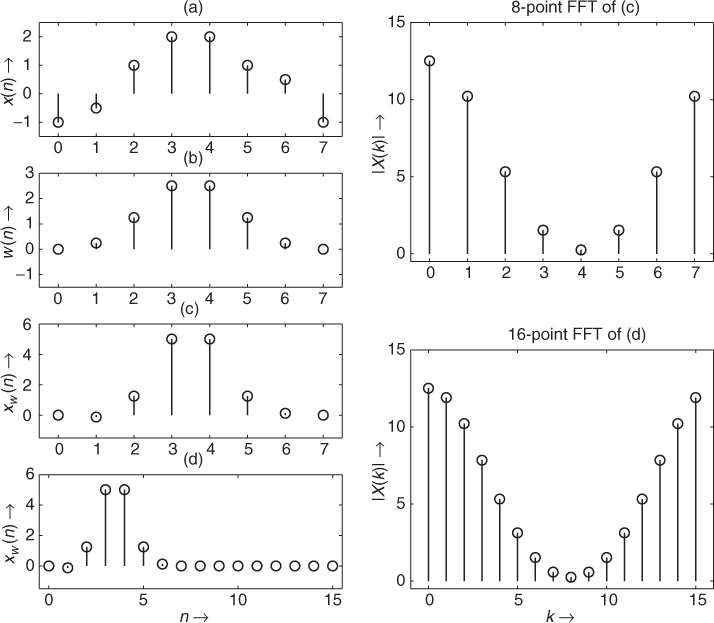
and weighting the N audio samples by the window function. This weighting is performed according to ![]() with 0 ≤ n ≤ N − 1 and then an FFT of the weighted signal is performed. The cosine weighted by a window and the corresponding spectrum is shown in the middle part of Figure 1.18. The lower part of Figure 1.18 shows a segment of an audio signal weighted by the Blackman window and the corresponding spectrum via a FFT. Figure 1.19 shows further simple examples for the reduction of the leakage effect and can be generated by the M-file 1.5.
with 0 ≤ n ≤ N − 1 and then an FFT of the weighted signal is performed. The cosine weighted by a window and the corresponding spectrum is shown in the middle part of Figure 1.18. The lower part of Figure 1.18 shows a segment of an audio signal weighted by the Blackman window and the corresponding spectrum via a FFT. Figure 1.19 shows further simple examples for the reduction of the leakage effect and can be generated by the M-file 1.5.
M-file 1.4 (figure1_18.m)
%Author: U. Zölzer
x=cos(2*pi*1000*(0:1:N-1)/44100)’;
figure(2)
W=blackman(N);
W=N*W/sum(W); % scaling of window
f=((0:N/2-1)/N)*FS;
xw=x.*W;
subplot(3,2,1);plot(0:N-1,x);
axis([0 1000 -1.1 1.1]);
title(’a) Cosine signal x(n)’)
subplot(3,2,3);plot(0:N-1,xw);axis([0 8000 -4 4]);
title(’c) Cosine signal x_w(n)=x(n) cdot w(n) with window’)
X=20*log10(abs(fft(x,N))/(N/2));
subplot(3,2,2);plot(f,X(1:N/2));
axis([0 10000 -80 10]);
ylabel(’X(f)’);
title(’b) Spectrum of cosine signal’)
Xw=20*log10(abs(fft(xw,N))/(N/2));
subplot(3,2,4);plot(f,Xw(1:N/2));
axis([0 10000 -80 10]);
ylabel(’X(f)’);
title(’d) Spectrum with Blackman window’)
s=u1(1:N).*W;
subplot(3,2,5);plot(0:N-1,s);axis([0 8000 -1.1 1.1]);
xlabel(’n ightarrow’);
title(’e) Audio signal x_w(n) with window’)
Sw=20*log10(abs(fft(s,N))/(N/2));
subplot(3,2,6);plot(f,Sw(1:N/2));
axis([0 10000 -80 10]);
ylabel(’X(f)’);
title(’f) Spectrum with Blackman window’)
xlabel(’f in Hz ightarrow’);
M-file 1.5 (figure1_19.m)
%Author: U. Zölzer
x=[-1 -0.5 1 2 2 1 0.5 -1];
w=blackman(8);
w=w*8/sum(w);
x1=x.*w’;
x2(16)=0;
x2(1:8)=x1;
subplot(421);
stem(0:1:7,x);axis([-0.5 7.5 -1.5 2.5]);
ylabel(’x(n) ightarrow’);
title(’a) 8 samples'),
subplot(423);
stem(0:1:7,w);axis([-0.5 7.5 -1.5 3]);
ylabel(’w(n) ightarrow’);
title(’b) 8 samples Blackman window’);
subplot(425);
stem(0:1:7,x1);axis([-0.5 7.5 -1.5 6]);
ylabel(’x_w(n) ightarrow’);
title(’c) x(n)cdot w(n)’);
subplot(427);
stem(0:1:15,x2);axis([-0.5 15.5 -1.5 6]);
xlabel(’n ightarrow’);ylabel(’x_w(n) ightarrow’);
title(’d) x(n)cdot w(n) + zero-padding’);
subplot(222);
stem(0:1:7,abs(fft(x1)));axis([-0.5 7.5 -0.5 15]);
ylabel(’|X(k)| ightarrow’);
title(’8-point FFT of c)’);
subplot(224);
stem(0:1:15,abs(fft(x2)));axis([-1 16 -0.5 15]);
xlabel(’k ightarrow’);ylabel(’|X(k)| ightarrow’);
title(’16-point FFT of d)’);
Figure 1.18 Spectrum analysis of digital signals: take N audio samples and perform an N point discrete Fourier transform to yield N samples of the spectrum of the signal starting from 0 Hz over ![]() where k is running from 0, 1, 2,…, N − 1. For (a)–(d),
where k is running from 0, 1, 2,…, N − 1. For (a)–(d), ![]() .
.
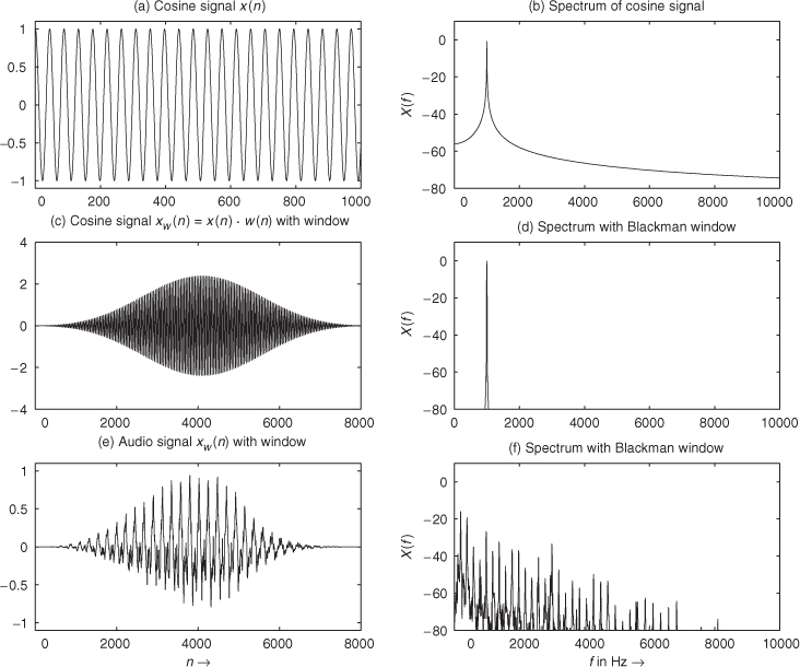
Figure 1.19 Reduction of the leakage effect by window functions: (a) the original signal, (b) the Blackman window function of length N = 8, (c) product x(n) · wB(n) with 0 ≤ n ≤ N − 1, (d) zero-padding applied to x(n) · wB(n) up to length N = 16 and the corresponding spectra are shown on the right side.
Spectrogram: Time-frequency Representation
A special time-frequency representation is the spectrogram which gives an estimate of the short-time, time-localized frequency content of the signal. To obtain the spectrogram the signal is split into segments of length N, which are multiplied by a window and an FFT is performed (see Figure 1.20). To increase the time-localization of the short-time spectra an overlap of the weighted segments can be used. A special visual representation of the short-time spectra is the spectrogram in Figure 1.21. Time increases linearly across the horizontal axis and frequency increases across the vertical axis. So each vertical line represents the absolute value |X(f)| over frequency by a grey-scale value (see Figure 1.21). Only frequencies up to half the sampling frequency are shown. The calculation of the spectrogram from a signal can be performed by the MATLAB function B = specgram(x,nFFT,Fs,window,nOverlap).
Figure 1.20 Short-time spectrum analysis by FFT.
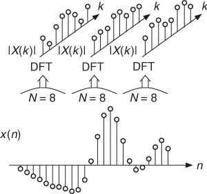
Figure 1.21 Spectrogram via FFT of weighted segments.

Another time-frequency representation of the short-time Fourier transforms of a signal x(n) is the waterfall representation in Figure 1.22, which can be produced by M-file 1.6 that calls the waterfall computation algorithm given by M-file 1.7.
Figure 1.22 Waterfall representation via FFT of weighted segments.

M-file 1.6 (figure1_22.m)
%Author: U. Zölzer
[signal,FS,NBITS]=wavread(’ton2’);
subplot(211);plot(signal);
subplot(212);
waterfspec(signal,256,256,512,FS,20,-100);
M-file 1.7 (waterfspec.m)
function yy=waterfspec(signal,start,steps,N,fS,clippingpoint,baseplane)
% Authors: J. Schattschneider, U. Zölzer
% waterfspec( signal, start, steps, N, fS, clippingpoint, baseplane)
%
% shows short-time spectra of signal, starting
% at k=start, with increments of STEP with N-point FFT
% dynamic range from -baseplane in dB up to 20*log(clippingpoint)
% in dB versus time axis
echo off;
if nargin<7, baseplane=-100; end
if nargin<6, clippingpoint=0; end
if nargin<5, fS=48000; end
if nargin<4, N=1024; end % default FFT
if nargin<3, steps=round(length(signal)/25); end
if nargin<2, start=0; end
windoo=blackman(N); % window - default
windoo=windoo*N/sum(windoo); % scaling
% Calculation of number of spectra nos
n=length(signal);
rest=n-start-N;
nos=round(rest/steps);
if nos>rest/steps, nos=nos-1; end
% vectors for 3D representation
x=linspace(0, fS/1000 ,N+1);
z=x-x;
cup=z+clippingpoint;
cdown=z+baseplane;
signal=signal+0.0000001;
% Computation of spectra and visual representation
for i=1:1:nos,
spek1=20.*log10(abs(fft(windoo.*signal(1+start+....
....i*steps:start+N+i*steps)))./(N)/0.5);
spek=[-200 ; spek1(1:N)];
spek=(spek>cup’).*cup’+(spek<=cup’).*spek;
spek=(spek<cdown’).*cdown’+(spek>=cdown’).*spek;
spek(1)=baseplane-10;
spek(N/2)=baseplane-10;
y=x-x+(i-1);
if i==1,
p=plot3(x(1:N/2),y(1:N/2),spek(1:N/2),’k’);
set(p,’Linewidth’,0.1);
end
pp=patch(x(1:N/2),y(1:N/2),spek(1:N/2),’w’,’Visible’,’on’);
set(pp,’Linewidth’,0.1);
end;
set(gca,’DrawMode’,’fast’);
axis([-0.3 fS/2000+0.3 0 nos baseplane-10 0]);
set(gca,’Ydir’,’reverse’);
view(12,40);
1.3.3 Digital Systems
A digital system is represented by an algorithm which uses the input signal x(n) as a sequence (stream) of numbers and performs mathematical operations upon the input signal such as additions, multiplications and delay operations. The result of the algorithm is a sequence of numbers or the output signal y(n). Systems which do not change their behavior over time and fulfill the superposition property [Orf96] are called linear time-invariant (LTI) systems. The input/output relations for a LTI digital system describe time-domain relations which are based on the following terms and definitions:
- Unit impulse, impulse response and discrete convolution;
- Algorithms and signal flow graphs.
For each of these definitions an equivalent description in the frequency domain exists, which will be introduced later.
Unit Impulse, Impulse Response and Discrete Convolution
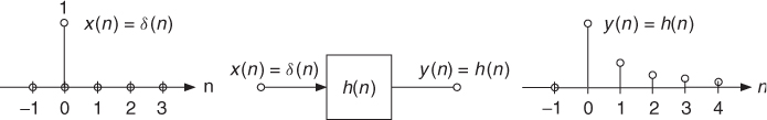
- Test signal: a very useful test signal for digital systems is the unit impulse
1.7
which is equal to one for n = 0 and zero elsewhere (see Figure 1.23).
- Impulse response: if we apply a unit-impulse function to a digital LTI system, the digital system will lead to an output signal y(n) = h(n), which is called the impulse response h(n) of the digital system. The digital LTI system is completely described by the impulse response, which is pointed out by the label h(n) inside the box, as shown in Figure 1.23.
- Discrete convolution: if we know the impulse response h(n) of a digital system, we can calculate the output signal y(n) from a freely chosen input signal x(n) by the discrete convolution formula given by
which is often abbreviated by the second term y(n) = x(n) * h(n). This discrete sum formula (1.8) represents an input–output relation for a digital system in the time domain. The computation of the convolution sum formula (1.8) can be achieved by the MATLAB function y=conv(x,h).
Figure 1.23 Impulse response h(n) as a time-domain description of a digital system.
Algorithms and Signal Flow Graphs
The above given discrete convolution formula shows the mathematical operations which have to be performed to obtain the output signal y(n) for a given input signal x(n). In the following we will introduce a visual representation called a signal flow graph which represents the mathematical input/output relations in a graphical block diagram. We discuss some example algorithms to show that we only need three graphical representations for the multiplication of signals by coefficients, delay and summation of signals.
- A delay of the input signal by two sampling intervals is given by the algorithm
1.9
and is represented by the block diagram in Figure 1.24.
- A weighting of the input signal by a coefficient a is given by the algorithm
1.10
and represented by a block diagram in Figure 1.25.
- The addition of two input signals is given by the algorithm
1.11

and represented by a block diagram in Figure 1.26.
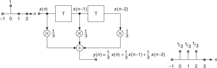
- The combination of the above algorithms leads to the weighted sum over several input samples, which is given by the algorithm
1.12
and represented by a block diagram in Fig. 1.27.
Figure 1.24 Delay of the input signal.
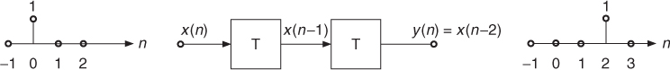
Figure 1.25 Weighting of the input signal.
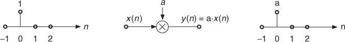
Figure 1.26 Addition of two signals x1(n) and x2(n).
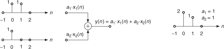
Figure 1.27 Simple digital system.
Transfer Function and Frequency Response
So far our description of digital systems has been based on the time-domain relationship between the input and output signals. We noticed that the input and output signals and the impulse response of the digital system are given in the discrete time domain. In a similar way to the frequency-domain description of digital signals by their spectra given in the previous subsection we can have a frequency-domain description of the digital system which is represented by the impulse response h(n). The frequency-domain behavior of a digital system reflects its ability to pass, reject and enhance certain frequencies included in the input signal spectrum. The common terms for the frequency-domain behavior are the transfer function H(z) and the frequency response H(f) of the digital system. Both can be obtained by two mathematical transforms applied to the impulse response h(n).
The first transform is the Z-Transform
1.13 
applied to the signal x(n) and the second transform is the discrete-time Fourier transform
1.14 
applied to the signal x(n). Both are related by the substitution z ↔ ejω. If we apply the Z-transform to the impulse response h(n) of a digital system according to
1.16 
we denote H(z) as the transfer function. The transfer function is of special interest as it relates the Z-transforms of input signal and output signal of the described system by
1.17 ![]()
If we apply the discrete-time Fourier transform to the impulse response h(n) we get
1.18 
Substituting (1.15) we define the frequency response of the digital system by
1.19 
Causal and Stable Systems
A realizable digital system has to fulfill the following two conditions:
- Causality: a discrete-time system is causal, if the output signal y(n) = 0 for n < 0 for a given input signal x(n) = 0 for n < 0. This means that the system cannot react to an input before the input is applied to the system.
- Stability: a digital system is stable if
1.20
holds. The sum over the absolute values of h(n) has to be less than a fixed number M2 < ∞.
The stability implies that the transfer function (Z-transform of impulse response) and the frequency response (discrete-time Fourier transform of impulse response) of a digital system are related by the substitution z ↔ ejω. Realizable digital systems have to be causal and stable systems. Some Z-transforms and their discrete-time Fourier transforms of a signal x(n) are given in Table 1.4.
Table 1.4 Z-transforms and discrete-time Fourier transforms of x(n)
| Signal | Z-transform | Discrete-time Fourier transform |
| x(n) | X(z) | X(ejω) |
| x(n − M) | z−M · X(z) | e−jωM · X(ejω) |
| δ(n) | 1 | 1 |
| δ(n − M) | z−M | e−jωM |
IIR and FIR Systems
IIR systems: A system with an infinite impulse response h(n) is called an IIR system. From the block diagram in Figure 1.28 we can read the difference equation
The output signal y(n) is fed back through delay elements and a weighted sum of these delayed outputs is summed up to the input signal x(n). Such a feedback system is also called a recursive system. The Z-transform of (1.21) yields
1.22 ![]()
1.23 ![]()
and solving for Y(z)/X(z) gives transfer function
1.24 ![]()
Figure 1.28 Simple IIR system with input signal x(n) and output signal y(n).
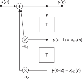
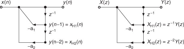
Figure 1.29 shows a special signal flow graph representation, where adders, multipliers and delay operators are replaced by weighted graphs.
Figure 1.29 Signal flow graph of digital system in Figure 1.28 with time-domain description in the left block diagram and corresponding frequency-domain description with Z-transform.
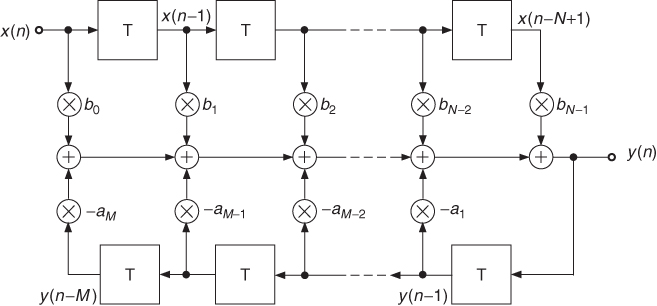
If the input delay line is extended up to N − 1 delay elements and the output delay line up to M delay elements according to Figure 1.30, we can write for the difference equation
1.25 
the Z-transform of the difference equation
1.26 
and the resulting transfer function
1.27 
Figure 1.30 IIR system.
The block processing approach for the IIR filter algorithm can be performed with the MATLAB/Octave function y = filter(b, a, x), where b and a are vectors with the filter coefficients as above and x contains the input signal.
A sample-by-sample processing approach for a second-order IIR filter algorithm is demonstrated by M-file 1.8.
M-file 1.8 (DirectForm01.m)
% Author: U. Zölzer
% Impulse response of 2nd order IIR filter
% Sample-by-sample algorithm
clear
% Coefficients for a high-pass
a=[1, -1.28, 0.47];
b=[0.69, -1.38, 0.69];
% Initialization of state variables
xh1=0;xh2=0;
yh1=0;yh2=0;
% Input signal: unit impulse
N=20; % length of input signal
x(N)=0;x(1)=1;
% Sample-by-sample algorithm
for n=1:N
y(n)=b(1)*x(n)+b(2)*xh1+b(3)*xh2 - a(2)*yh1 - a(3)*yh2;
xh2=xh1;xh1=x(n);
yh2=yh1;yh1=y(n);
end;
% Plot results
subplot(2,1,1)
stem(0:1:length(x)-1,x,’.’);axis([-0.6 length(x)-1 -1.2 1.2]);
xlabel(’n ightarrow’);ylabel(’x(n) ightarrow’);
subplot(2,1,2)
stem(0:1:length(x)-1,y,’.’);axis([-0.6 length(x)-1 -1.2 1.2]);
xlabel(’n ightarrow’);ylabel(’y(n) ightarrow’);
Computation of the frequency response based on the coefficients of the transfer function ![]() can be made with the MATLAB/Octave function freqz(b, a), while the poles and zeros can be determined with zplane(b, a).
can be made with the MATLAB/Octave function freqz(b, a), while the poles and zeros can be determined with zplane(b, a).
FIR systems: A system with a finite impulse response h(n) is called an FIR system. From the block diagram in Figure 1.31 we can read the difference equation
The input signal x(n) is fed forward through delay elements and a weighted sum of these delayed inputs is summed up to the input signal y(n). Such a feed-forward system is also called a non-recursive system. The Z-transform of (1.28) yields
1.29 ![]()
1.30 ![]()
and solving for Y(z)/X(z) gives transfer function
1.31 ![]()
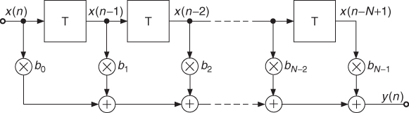
A general FIR system in Figure 1.32 consists of a feed-forward delay line with N − 1 delay elements and has the difference equation
1.32 
The finite impulse response is given by
1.33 
which shows that each impulse of h(n) is represented by a weighted and shifted unit impulse. The Z-transform of the impulse response leads to the transfer function
The time-domain algorithms for FIR systems are the same as those for IIR systems with the exception that the recursive part is missing. The previously introduced M-files for IIR systems can be used with the appropriate coefficients for FIR block processing or sample-by-sample processing.
Figure 1.31 Simple FIR system with input signal x(n) and output signal y(n).
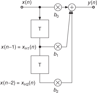
Figure 1.32 FIR system.
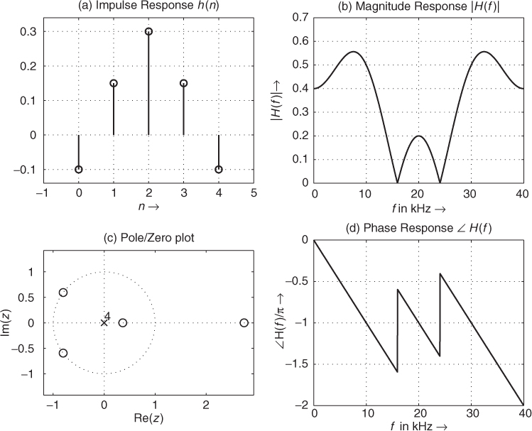
The computation of the frequency response H(f) = |H(f)| · ej∠H(f) (|H(f)| magnitude response, φ = ∠H(f) phase response) from the Z-transform of an FIR impulse response according to (1.34) is shown in Figure 1.33 and is calculated by the following M-file 1.9.
Figure 1.33 FIR system: (a) impulse response, (b) magnitude response, (c) pole/zero plot and (d) phase response (sampling frequency ![]() ).
).
M-file 1.9 (figure1_33.m)
function magphasresponse(h)
% Author: U. Zölzer
FS=40000;
fosi=10;
if nargin==0
h=[-.1 .15 .3 .15 -.1];
end
hmax=max(h);
hmin=min(h);
dh=hmax-hmin;
hmax=hmax+.1*dh;
hmin=hmin-.1*dh;
N=length(h);
% denominator polynomial:
a=zeros(1,N);
a(1)=1;
subplot(221)
stem(0:N-1,h)
axis([-1 N, hmin hmax])
title(’a) Impulse Response h(n)’,’Fontsize’,fosi);
xlabel(’n ightarrow’,’Fontsize’,fosi)
grid on;
subplot(223)
zplane(h,a)
title(’c) Pole/Zero plot’,’Fontsize’,fosi);
xlabel(’Re(z)’,’Fontsize’,fosi)
ylabel(’Im(z)’,’Fontsize’,fosi)
subplot(222)
[H,F]=freqz(h,a,1024,’whole’,FS);
plot(F/1000,abs(H))
xlabel(’f in kHz ightarrow’,’Fontsize’,fosi);
ylabel(’|H(f)| ightarrow’,’Fontsize’,fosi);
title(’b) Magnitude response |H(f)|’,’Fontsize’,fosi);
grid on;
subplot(224)
plot(F/1000,unwrap(angle(H))/pi)
xlabel(’f in kHz ightarrow’,’Fontsize’,fosi)
ylabel(’angle H(f)/pi ightarrow’,’Fontsize’,fosi)
title(’d) Phase Response angle H(f)’,’Fontsize’,fosi);
grid on;