
14.3 Source Separation from Single-channel Signals
Separation of sources from single-channel (monophonic) mixtures is particularly challenging. If we have two or more microphones, we have seen earlier in this chapter that we can use information on relative amplitudes or relative time delays to identify the sources and to help us perform the separation. But with only one microphone, this information is not available. Instead, we must use information about the structure of the source signals to identify and separate the different components.
For example, one popular approach to the single-channel source separation problem is to use non-negative matrix factorization (NMF) of the Short Time Fourier Transform (STFT) power spectrogram of the audio signal. This method attempts to identify consistent spectral patterns in the different source signals, allowing these patterns to be associated with the different sources, then allowing separation of the audio signals. As well as NMF, we shall see that methods based on sinusoidal modeling and probabilistic modeling have also been proposed to tackle this difficult problem.
14.3.1 Source Separation Using Non-negative Matrix Factorization
Suppose that our mixture signal is composed of a weighted mixture of simple source objects, each with a fixed power spectrum ![]() , and where the relative energy of the pth object in the nth frame is given by spn ≥ 0. Then the activity of each object has a spectrum of xpn = apspn at frame n. If we then assume that the source signal objects have random phase, so that the spectral energy due to each source object approximately adds in each time-frequency spectral bin, then the spectrum of the mixture will be approximately given by
, and where the relative energy of the pth object in the nth frame is given by spn ≥ 0. Then the activity of each object has a spectrum of xpn = apspn at frame n. If we then assume that the source signal objects have random phase, so that the spectral energy due to each source object approximately adds in each time-frequency spectral bin, then the spectrum of the mixture will be approximately given by
14.46 ![]()
or in matrix notation
14.47 ![]()
where X is the mixture spectrogram, A = [ap] is the matrix of spectra for each source, and S = [spn] is the matrix of relative source energies in each frame. Since each of the matrices X, A and S represent amounts of energy, they are all non-negative.
In single-channel source separation, we only observe the mixture signal with its corresponding non-negative spectrogram X. But, since A and S are also non-negative, we can use non-negative matrix factorization (NMF) [LS99] to approximately recover A and S from X.
Non-negative Matrix Factorization (NMF)
In its simplest form, NMF attempts to minimize a cost function J = D(V;WH) between a non-negative matrix V and a product of two non-negative matrices WH. For example, we could use the Euclidean cost function
14.48 ![]()
or the (generalized) Kullback–Leibler divergence,
and search for a minimum of J using, e.g., a gradient descent method. In fact we can simplify things a little, since there is a scaling ambiguity between W and H, so we are free to normalize the columns of W to sum to unity, ∑ωwωp = 1. Lee and Seung [LS99] introduced a simple parameter-free “multiplicative update” method to perform this optimization;
14.50 
where this procedure optimizes the KL divergence (14.49).
Figure 14.17(a) shows a simple example where we have two sources w1 and w2, each consisting of a single frequency, with their activations over time given by h1 and h2. Smaragdis and Brown [SB03] applied this type of NMF to polyphonic music transcription, where they were looking to identify the spectra (wp) and activities (hp) of, e.g., individual piano notes.
Figure 14.17 Simple example of non-negative matrix factorization.
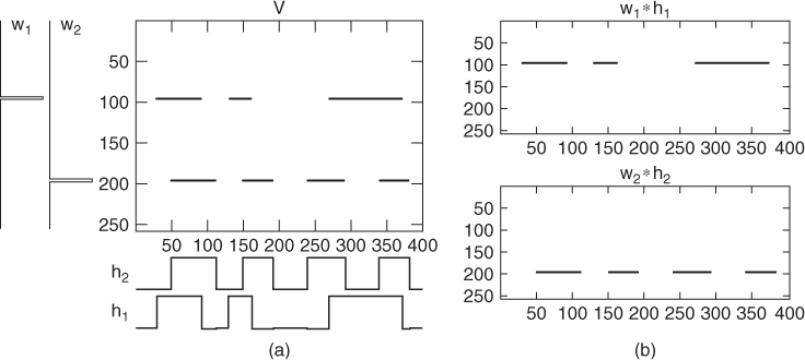
For simple sources such as individual notes, we could use the separate products ![]() as an estimate of the spectrogram of the original source. We could then transform back to the time domain simply by using the phases in the mixture spectrum as estimates of the phases of the original sources. However, in practice this approach can be limited, since it assumes that: (a) the source spectrum is unchanging over time and (b) real sources can often change their pitch, which would produce many separate “sources” from NMF [WP06].
as an estimate of the spectrogram of the original source. We could then transform back to the time domain simply by using the phases in the mixture spectrum as estimates of the phases of the original sources. However, in practice this approach can be limited, since it assumes that: (a) the source spectrum is unchanging over time and (b) real sources can often change their pitch, which would produce many separate “sources” from NMF [WP06].
Convolutive NMF
Real sources tend to change their spectrum over time, for example with the high-frequency components decaying faster than the low-frequency components. To account for this, Virtanen [Vir04] and Smaragdis [Sma04, Sma07] introduced a convolutive NMF approach, known as non-negative matrix factor deconvolution (NMFD). Here, each source is no longer represented by a single spectrum, but instead by a typical spectrogram which reflects how the spectrum of the source changes over time.
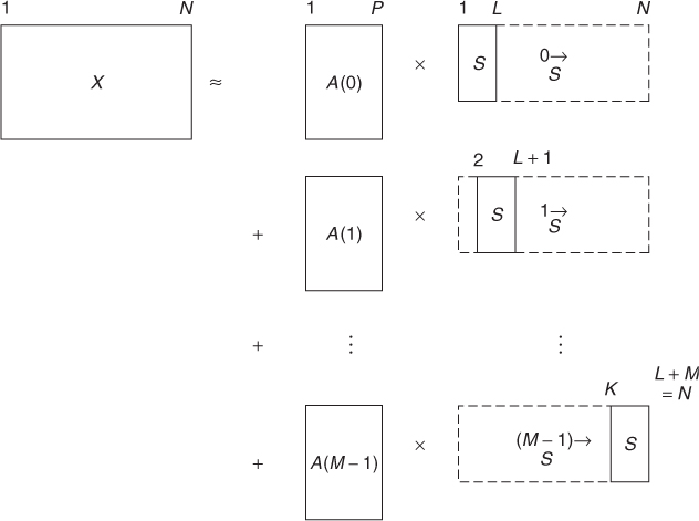
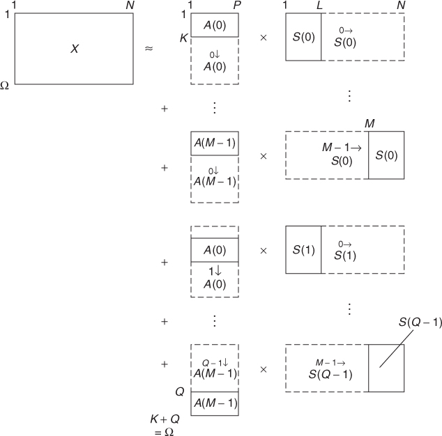
For NMFD, our model becomes
14.51 ![]()
which we can write in a matrix form as (Figure 14.18)
14.52 
where the ![]() matrix notation means that the matrix is shifted m places to the right
matrix notation means that the matrix is shifted m places to the right
14.53 ![]()
Smaragdis [Sma04] applied NMFD to separation of drum sounds, using it to separate bass drum, snare drum and hi-hat from a mixture.
Figure 14.18 Convolutive NMF model for Non-negative Matrix Factor Deconvolution (NMFD).
2D Convolutive NMF
The convolutive approach, NMFD, relies on each drum sound having a characteristic spectrogram that evolves in a very similar way each time that sound plays. However, pitched instruments have a spectrum that is typically composed of spectral lines that change as the pitch of the note changes. To deal with this, Schmidt and Mørup [SM06] extended the (time-) convolutive NMF approach to a 2D convolutive NMF method, NMF2D. NMF2D uses a spectrogram with a log-frequency scale, so that pitch changes become a vertical shift, while time changes are a horizontal shift (as for NMFD).
The model then becomes
14.54 ![]()
which we can write in a matrix convolution form as (Figure 14.19)
14.55 
where the ![]() matrix notation indicates that the contents of the matrix are shifted q places down
matrix notation indicates that the contents of the matrix are shifted q places down
14.56 ![]()
Schmidt and Mørup [SM06] used NMF2D to separate trumpet from piano sounds.
Figure 14.19 Two-dimensional convolutive NMF model (NMF2D).
14.3.2 Structural Cues
Sinusoidal Modeling
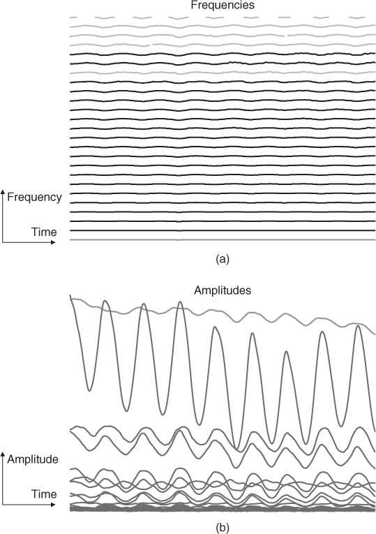
Sinusoidal modeling has solid mathematical, physical and physiological bases. It derives from Helmholtz's research and is rooted in Fourier's theorem, which states that any periodic function can be modeled as a sum of sinusoids at various amplitudes and harmonically related frequencies. Here we will consider the sinusoidal model under its most general expression, which is a sum of sinusoids (the partials) with time-varying amplitudes and frequencies not necessarily harmonically related. The associated representation is in general orthogonal (the partials are independent) and sparse (a few amplitude and frequency parameters can be sufficient to describe a sound consisting of many samples), thus very computationally efficient. Each partial is a pure tone, part of the complex sound (see Figure 14.20). The partials are sound structures very important both from the production (acoustics) and perception (psychoacoustics) points of view. In acoustics, they correspond to the modes of musical instruments, the superpositions of vibration modes being the solutions of the equations for vibrating systems (e.g., strings, bars, membranes). In psychoacoustics, the partials correspond to tonal components of high energy, thus very important for masking phenomena. The fact that the auditory system is well adapted to the acoustical environment seems quite natural.
Figure 14.20 The evolutions of the partials of an alto saxophone over ≈1.5 second. The frequencies (a) and amplitudes (b) are displayed as functions of time (horizontal axis).
From a perceptual point of view, some partials belong to the same sound entity if they are perceived by the human auditory system as a unique sound when played together. There are several criteria that lead to this perceptual fusion. After Bregman [Bre90], we consider:
- The common onsets/offsets of the spectral components.
- The spectral structure of the sound, taking advantage of harmonic relations.
- The correlated variations of the time evolutions of these spectral parameters.
- The spatial location, estimated by a localization algorithm.
All these criteria allow us to classify the spectral components. Since this is done according to the perception, the classes we obtain should be the sound entities of the auditory scene. And the organization of these sound entities in time should give the musical structure. Music transcription is then possible by extracting musical parameters from these sound entities. But an advantage over standard music information retrieval (MIR) approaches is that here the sound entities are still available for transformation and resynthesis of a modified version of the music.
The use of each criterion gives a different way to classify the partials. One major problem is to be able to fuse these heterogeneous criteria, to obtain a unique classification method. Another problem is to incorporate this structuring within the analysis chain, to obtain a partial tracking algorithm with multiple criteria that would track classes of partials (entities) instead of individual partials, and thus should be more robust. Finding solutions to these problems are major research directions.
Common Onsets
As noted by Hartmann [Har88], the common onset (birth) of partials plays a preponderant role in our perception of sound entities. From the experiences of Bregman and Pinker [BP78] and Gordon [Gor84], the partials should appear within a short time window of around 30 ms (corresponding to a number of γ consecutive frames, see below), else they are likely to be heard separately. Many onset-detection methods are based on the variation in time of the amplitude or phase of the signal (see [BDA+05] for a survey). Lagrange [Lag04] proposes an algorithm based on the D measure defined as
14.58 
where ap is the amplitude of the partial p, ![]() p is its mean value, and
p is its mean value, and ![]() p[n] is 1 if the partial is born in the [n − γ,n + γ] interval and 0 otherwise. Thanks to this measure, it seems that we can identify the onsets of notes even if their volume fades in slowly (see Figure 14.21), leading to a better structuring of the sound entities (see Figure 14.22).
p[n] is 1 if the partial is born in the [n − γ,n + γ] interval and 0 otherwise. Thanks to this measure, it seems that we can identify the onsets of notes even if their volume fades in slowly (see Figure 14.21), leading to a better structuring of the sound entities (see Figure 14.22).
Figure 14.21 Examples of note onset detection using two different measures: (a) the difference in amplitude between consecutive frames and (b) the D measure of Equation (14.57). The true onsets—annotated manually—are displayed as vertical bars. Our method manages to identify correctly the note onsets, even if the volume of the note fades in slowly (see around frame 200).
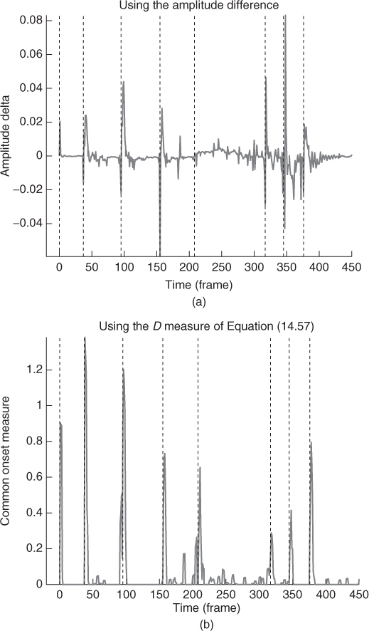
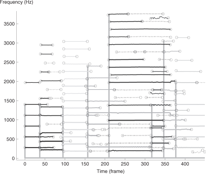
Figure 14.22 Result of the structuring of the partials in sound entities using the common onset criterion on the example of Figure 14.21.
Simple-and Poly-harmonic Structures
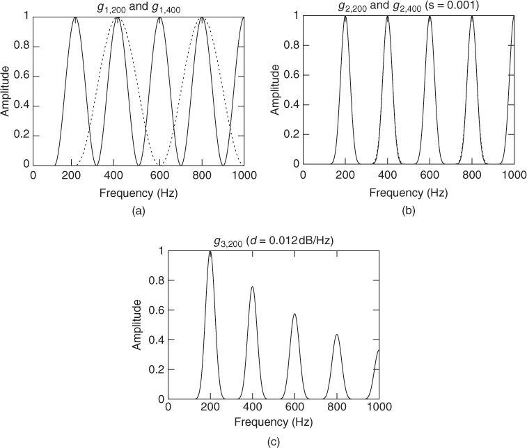
The earliest attempts at acoustical entity identification and separation consider harmonicity as the sole cue for group formation. Some rely on a prior detection of the fundamental frequency [Gro96] and others consider only the harmonic relation of the frequencies [Kla03]. A classic approach is to perform a correlation of the short-term spectrum with some template, which should be a periodic function, of period F–the fundamental frequency under investigation. Such a template can be built using the expression of the Hann window
14.59 ![]()
where f is the frequency and F is the fundamental. However, the problem with these templates is that the width of the template peaks depend on F (see Figure 14.23.a). For a constant peak selectivity, we can propose another function
14.60 ![]()
where s ∈ (0, 1] allows us to tune this selectivity (see Figure 14.23.b). But this template is still too far from the typical structure of musical sounds, whose spectral envelope (in dB) is often a linear function of the frequency (in Hz), see [Kla03]. Thus, we can consider
14.61 ![]()
where d is the slope of the spectral envelope, in dB per Hz (see Figure 14.23.(c)). Multi-pitch estimation is still an active research area, and yet our simple approach gives very good results, especially when the s and d parameters can be learned from a database. However, many musical instruments are not perfectly harmonic, and the template should ideally also depend on the inharmonicity factor in the case of inharmonic sounds.
Figure 14.23 Three kinds of templates for the extraction of harmonic structures: (a) simple periodic function, (b) modified version for a constant peak selectivity, and (c) modified version for a more realistic spectral envelope.
Similar Evolutions
According to the work of McAdams [McA89], a group of partials is perceived as a unique sound entity only if the variations of these partials are correlated, whether the sound is harmonic or not.
An open problem is the quest for a relevant dissimilarity between two elements (the partials), that is a dissimilarity which is low for elements of the same class (sound entity) and high for elements that do not belong to the same class. It turns out that the auto-regressive (AR) modeling of the parameters of the partials is a good candidate for the design of a robust dissimilarity metric.
Let ωp be the frequency vector of the partial p. According to the AR model, the sample ωp[n] can be approximated as a linear combination of past samples
14.62 
where ep[n] is the prediction error. The coefficients cp[k] model the predictable part of the signal and it can be shown that these coefficients are scale invariant. Conversely the non-predictable part ep[n] is not scale invariant. For each frequency vector ωp, we compute a vector cp[k] of four AR coefficients with the Burg method. Although the direct comparison of the AR coefficients computed from the two vectors ωp and ωq is generally not relevant, the spectrum of these coefficients may be compared. The Itakura distortion measure [Ita75], issued from the speech recognition community can be considered:
14.63 ![]()
where
14.64 
Another approach may be considered. Indeed, the amount of error done by modeling the vector ωp by the coefficients computed from vector ωq may indicate the dissimilarity of these two vectors. Let us introduce a new notation ![]() , the cross-prediction error defined as the residual signal of the filtering of the vector ωp with cq
, the cross-prediction error defined as the residual signal of the filtering of the vector ωp with cq
14.65 
The principle of the dissimilarity dσ is to combine the two dissimilarities ![]() and
and ![]() to obtain a symmetrical one:
to obtain a symmetrical one:
14.66 ![]()
Given two vectors ωp and ωq to be compared, the coefficients cp and cq are computed to minimize the power of the respective prediction errors ep and eq. If the two vectors ωp and ωq are similar, the power of the cross-prediction errors ![]() and
and ![]() will be as weak as those of ep and eq. We can consider another dissimilarity
will be as weak as those of ep and eq. We can consider another dissimilarity ![]() defined as the ratio between the sum of the crossed prediction errors and the sum of the direct prediction errors:
defined as the ratio between the sum of the crossed prediction errors and the sum of the direct prediction errors:
14.67 ![]()
Lagrange [Lag05] shows that the metrics based on AR modeling perform quite well.
14.3.3 Probabilistic Models
We can also view the source separation problem as a probabilistic inference problem [VJA+10]. In outline, one uses a probabilistic model p(x|s1, s2) for the observed mixture x from two sources s1 and s2, and then attempt to find the original sources given the mixture. This is typically done using the maximum a posteriori (MAP) criterion
14.68 ![]()
using the Bayesian formulation p(s1, s2|x)∝p(x|s1, s2)p(s1)p(s2), where the sources s1 and s2 are assumed to be independent, although other criteria, such as the posterior mean (PM) are also possible.
Benaroya et al. [BBG06] use this probabilistic approach, modeling the sources using Gaussian mixture models (GMMs) and Gaussian scaled mixture models (GSMMs). A GSMM is a mixture of Gaussian scaled densities, each of which corresponds to a random variable of the form ![]() , where g is a Gaussian with variance σ2 and a is a non-negative scalar random variable with prior density p0(a).
, where g is a Gaussian with variance σ2 and a is a non-negative scalar random variable with prior density p0(a).
They demonstrated their approach on separation of jazz tracks, considering “piano + bass” as one source and drums as another source. The model parameters were trained on a CD containing the separated tracks. This type of CD was originally designed for people to learn how to play jazz, but is also convenient for this type of experiment since it contains separated sources which make a coherent piece of music when mixed together. They found good performance with about 8 or 16 components, although this depended on the particular model used and the estimation method (MAP or PM). For more details about other probabilistic modeling-based approaches, see [VJA+10].