
2.2.1 Filter Classification in the Frequency Domain
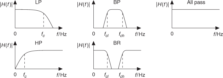
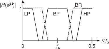
The various types of filters can be defined according to the following classification (see Figure 2.1):
- Lowpass (LP) filters select low frequencies up to the cut-off frequency fc and attenuate frequencies higher than fc. Additionally, a resonance may amplify frequencies around fc.
- Highpass (HP) filters select frequencies higher than fc and attenuate frequencies below fc, possibly with a resonance around fc.
- Bandpass (BP) filters select frequencies between a lower cut-off frequency fcl and a higher cut-off frequency fch. Frequencies below fcl and frequencies higher than fch are attenuated.
- Bandreject (BR) filters attenuate frequencies between a lower cut-off frequency fcl and a higher cut-off frequency fch. Frequencies below fcl and frequencies higher than fch are passed.
- Allpass filters pass all frequencies, but modify the phase of the input signal.
Figure 2.1 Filter classification.
The lowpass with resonance is very often used in computer music to simulate an acoustical resonating structure; the highpass filter can remove undesired very low frequencies; the bandpass can produce effects such as the imitation of a telephone line or of a mute on an acoustical instrument; the bandreject can divide the audible spectrum into two bands that seem to be uncorrelated.
2.2.2 Canonical Filters
There are various ways to implement a filter, the simplest being the canonical filter, as shown in Figure 2.2 for a second-order filter, which can be implemented by the difference equations
2.1 ![]()
and leads to the transfer function
2.3 ![]()
Figure 2.2 Canonical second-order digital filter.
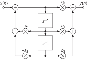
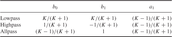
By setting a2 = b2 = 0, this reduces to a first-order filter which, can be used to implement an allpass, lowpass or highpass with the coefficients of Table 2.1 where K depends on the cut-off frequency fc by
2.4 ![]()
For the allpass filter, the coefficient K likewise controls the frequency fc when −90° phase shift is reached.
Table 2.1 Coefficients for first-order filters
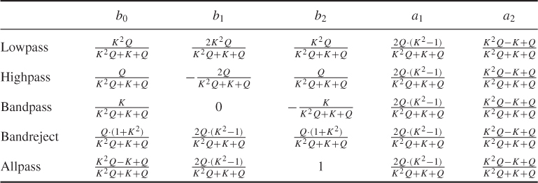
For the second-order filters with coefficients shown in Table 2.2, in addition to the cut-off frequency (for lowpass and highpass) or the center frequency (for bandpass, bandreject and allpass) we additionally need the Q factor with slightly different meanings for the different filter types:
- For the lowpass and highpass filters, it controls the height of the resonance. For
 , the filter is maximally flat up to the cut-off frequency; for lower Q, it has higher pass-band attenuation, while for higher Q, amplification around fc occurs.
 - For the bandpass and bandreject filters, it is related to the bandwidth fb by
 , i.e., it is the inverse of the relative bandwidth
  .
. - For the allpass filter, it likewise controls the bandwidth, which here depends on the points where ±90° phase shift relative to the −180° phase shift at fc are reached.
Table 2.2 Coefficients for second-order filters
While the canonical filters are relatively simple, the calculation of their coefficients from parameters like cut-off frequency and bandwidth is not. In the following, we will therefore study filter structures that are slightly more complicated, but allow for easier parameterization.
2.2.3 State Variable Filter
A nice alternative to the canonical filter structure is the state variable filter shown in Figure 2.3 [Cha80], which combines second-order lowpass, bandpass and highpass for the same fc and Q. Its difference equation is given by
2.5 ![]()
2.6 ![]()
2.7 ![]()
where yl(n), yb(n) and yh(n) are the outputs of lowpass, bandpass, and highpass, respectively. The tuning coefficients F1 and Q1 are related to the tuning parameters fc and Q by
2.8 ![]()
It can be shown that the transfer function of lowpass, bandpass, and highpass, respectively, are
2.9 ![]()
2.10 ![]()
2.11 ![]()
with r = F1 and q = 1 − F1Q1.
Figure 2.3 Digital state variable filter.
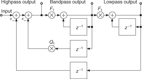
This structure is particularly effective not only as far as the filtering process is concerned, but above all because of the simple relations between control parameters and tuning coefficients. One should consider the stability of this filter, because at higher cut-off frequencies and smaller Q factors it becomes unstable. A “usability limit” given by F1 < 2 − Q1 assures the stable operation of the state variable implementation [Dut91, Die00]. In most musical applications, however, it is not a problem because the tuning frequencies are usually small compared to the sampling frequency and the Q factor is usually set to sufficiently high values [Dut89a, Dat97a]. This filter has proven its suitability for a large number of applications. The nice properties of this filter have been exploited to produce endless glissandi out of natural sounds and to allow smooth transitions between extreme settings [Dut89b, m-Vas93]. It is also used for synthesizer applications [Die00].
2.2.4 Normalization
Filters are usually designed in the frequency domain and as a consequence, they are expected to primarily affect the frequency content of the signal. However, the side effect of loudness modification must not be forgotten because of its importance for the practical use of the filter. The filter might produce the right effect, but the result might be useless because the sound has become too weak or too strong. The method of compensating for these amplitude variations is called normalization. Normalization is performed by scaling the filter such that the norm
2.12 
where typically L2 or ![]() are used [Zöl05]. To normalize the loudness of the signal, the L2 norm is employed. It is accurate for broadband signals and fits many practical musical applications. L∞ normalizes the maximum of the frequency response and avoids overloading the filter. With a suitable normalization scheme the filter can prove to be very easy to handle whereas with the wrong normalization, the filter might be rejected by musicians because they cannot operate it.
are used [Zöl05]. To normalize the loudness of the signal, the L2 norm is employed. It is accurate for broadband signals and fits many practical musical applications. L∞ normalizes the maximum of the frequency response and avoids overloading the filter. With a suitable normalization scheme the filter can prove to be very easy to handle whereas with the wrong normalization, the filter might be rejected by musicians because they cannot operate it.
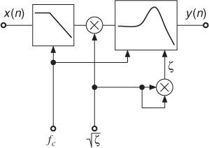
The normalization of the state variable filter has been studied in [Dut91], where several effective implementation schemes are proposed. In practice, a first-order lowpass filter that processes the input signal will perform the normalization in fc and an amplitude correction in ![]() will normalize in ζ (see Figure 2.4). This normalization scheme allows us to operate the filter with damping factors down to 10−4 where the filter gain reaches about 74 dB at fc.
will normalize in ζ (see Figure 2.4). This normalization scheme allows us to operate the filter with damping factors down to 10−4 where the filter gain reaches about 74 dB at fc.
Figure 2.4 L2-normalization in fc and ζ for the state variable filter.
2.2.5 Allpass-based Filters
In this subsection we introduce a special class of parametric filter structures for lowpass, highpass, bandpass and bandreject filter functions. Parametric filter structures denote special signal flow graphs where a coefficient inside the signal flow graph directly controls the cut-off frequency and bandwidth of the corresponding filter. These filter structures are easily tunable by changing only one or two coefficients. They play an important role for real-time control with minimum computational complexity.
The basis for parametric first- and second-order IIR filters is the first- and second-order allpass filter. We will first discuss the first-order allpass and show simple lowpass and highpass filters, which consist of a tunable allpass filter together with a direct path.
First-order Allpass
A first-order allpass filter is given by the transfer function (see 2.2.2)
2.14 ![]()
and the corresponding difference equation
2.15 ![]()
which can be realized by the block diagram shown in Figure 2.5.
Figure 2.5 Block diagram for a first-order allpass filter.
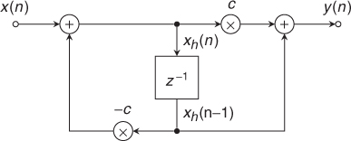
The magnitude/phase response and the group delay of a first-order allpass are shown in Figure 2.6. The magnitude response is equal to one and the phase response is approaching −180° for high frequencies. The group delay shows the delay of the input signal in samples versus frequency. The coefficient c in (2.13) controls the frequency where the phase response passes −90° (see Figure 2.6).
Figure 2.6 First-order allpass filter with fc = 0.1 · fS.
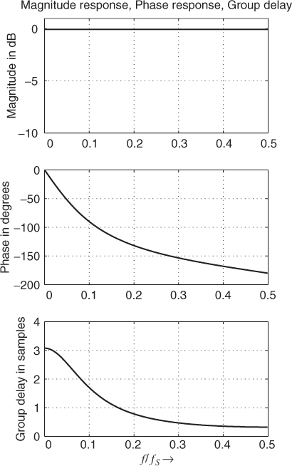
For simple implementations a table with a number of coefficients for different cut-off frequencies is sufficient, but even for real-time applications this structure offers very few computations. In the following we use this first-order allpass filter to perform low/highpass filtering.
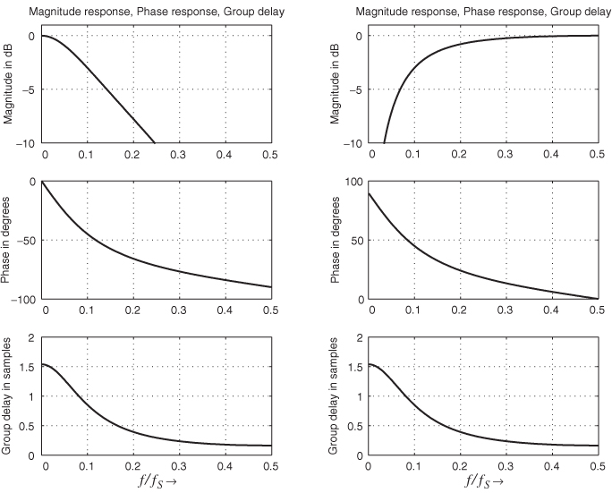
First-order Low/highpass
A first-order lowpass/highpass filter can be achieved by adding or subtracting (+/−) the output signal from the input signal of a first-order allpass filter. As the output signal of the first-order allpass filter has a phase shift of −180° for high frequencies, this operation leads to low/highpass filtering. The transfer function of a lowpass/highpass filter is then given by
2.17 ![]()
2.18 ![]()
2.19 ![]()
where a tunable first-order allpass A(z) with tuning parameter c is used. The plus sign (+) denotes the lowpass operation and the minus sign (−) the highpass operation. The block diagram in Figure. 2.7 represents the operations involved in performing the low/highpass filtering. The allpass filter can be implemented by the difference equation (2.16), as shown in Figure 2.5 to obtain the lowpass implementation of M-file 2.1.
M-file 2.1 (aplowpass.m)
function y = aplowpass (x, Wc)
% y = aplowpass (x, Wc)
% Author: M. Holters
% Applies a lowpass filter to the input signal x.
% Wc is the normalized cut-off frequency 0<Wc<1, i.e. 2*fc/fS.
c = (tan(pi*Wc/2)-1) / (tan(pi*Wc/2)+1);
xh = 0;
for n = 1:length(x)
xh_new = x(n) - c*xh;
ap_y = c * xh_new + xh;
xh = xh_new;
y(n) = 0.5 * (x(n) + ap_y); % change to minus for highpass
end;
Figure 2.7 Block diagram of a first-order low/highpass filter.
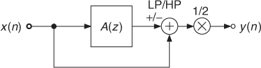
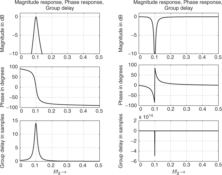
The magnitude/phase response and group delay are illustrated for low- and highpass filtering in Figure 2.8. The −3 dB point of the magnitude response for lowpass and highpass is passed at the cut-off frequency. With the help of the allpass subsystem in Figure 2.7, tunable first-order low- and highpass systems are achieved.
Figure 2.8 First-order low/highpass filter with fc = 0.1fS.
Second-order Allpass
The implementation of tunable bandpass and bandreject filters can be achieved with a second-order allpass filter. The transfer function of a second-order allpass filter is given by
2.20 ![]()
2.21 ![]()
2.22 ![]()
with the corresponding difference equations (compare Section 2.2.2)
2.23 ![]()
2.24 ![]()
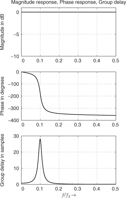
The parameter d adjusts the center frequency and the parameter c the bandwidth. The magnitude/phase response and the group delay of a second-order allpass are shown in Figure 2.9. The magnitude response is again equal to one and the phase response approaches −360° for high frequencies. The cut-off frequency fc determines the point on the phase curve where the phase response passes −180°. The width or slope of the phase transition around the cut-off frequency is controlled by the bandwidth parameter fb.
Figure 2.9 Second-order allpass filter with fc = 0.1fS and fb = 0.022fS.
Second-order Bandpass/bandreject
Second-order bandpass and bandreject filters can be described by the following transfer function
2.25 ![]()
2.26 ![]()
2.27 ![]()
2.28 ![]()
where a tunable second-order allpass A(z) with tuning parameters c and d is used. The minus sign (−) denotes the bandpass operation and the plus sign (+) the bandreject operation. The block diagram in Figure 2.10 shows the bandpass and bandreject filter implementation based on a second-order allpass subsystem, M-file 2.2 shows the corresponding MATLAB® code. The magnitude/phase response and group delay are illustrated in Figure 2.11 for both filter types.
M-file 2.2 (apbandpass.m)
function y = apbandpass (x, Wc, Wb)
% y = apbandpass (x, Wc, Wb)
% Author: M. Holters
% Applies a bandpass filter to the input signal x.
% Wc is the normalized center frequency 0<Wc<1, i.e. 2*fc/fS.
% Wb is the normalized bandwidth 0<Wb<1, i.e. 2*fb/fS.
c = (tan(pi*Wb/2)-1) / (tan(pi*Wb/2)+1);
d = -cos(pi*Wc);
xh = [0, 0];
for n = 1:length(x)
xh_new = x(n) - d*(1-c)*xh(1) + c*xh(2);
ap_y = -c * xh_new + d*(1-c)*xh(1) + xh(2);
xh = [xh_new, xh(1)];
y(n) = 0.5 * (x(n) - ap_y); % change to plus for bandreject
end;
Figure 2.10 Second-order bandpass and bandreject filter.
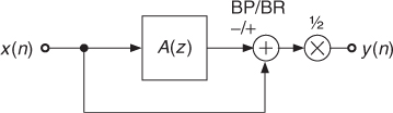
Figure 2.11 Second-order bandpass/bandreject filter with fc = 0.1fS and fb = 0.022fS.
2.2.6 FIR Filters
Introduction
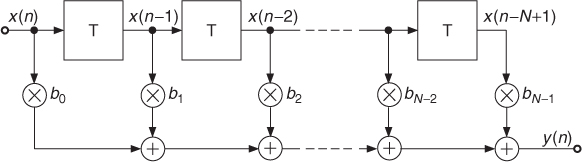
The digital filters that we have seen before are said to have an infinite impulse response. Because of the feedback loops within the structure, an input sample will excite an output signal whose duration is dependent on the tuning parameters and can extend over a fairly long period of time. There are other filter structures without feedback loops (Figure 2.12). These are called finite impulse response filters (FIR), because the response of the filter to a unit impulse lasts only for a fixed period of time. These filters allow the building of sophisticated filter types where strong attenuation of unwanted frequencies or decomposition of the signal into several frequency bands is necessary. They typically require higher filter orders and hence more computing power than IIR structures to achieve similar results, but when they are implemented in the form known as fast convolution they become competitive, thanks to the FFT algorithm. It is rather unwieldy to tune these filters interactively. As an example, let us briefly consider the vocoder application. If the frequency bands are fixed, then the FIR implementation can be most effective but if the frequency bands have to be subtly tuned by a performer, then the IIR structures will certainly prove superior [Mai97]. However, the filter structure in Figure 2.12 finds widespread applications for head-related transfer functions and the approximation of first room reflections, as will be shown in Chapter 5. For applications where the impulse response of a real system has been measured, the FIR filter structure can be used directly to simulate the measured impulse response.
Figure 2.12 Finite impulse response filter.
Signal Processing
The output/input relation of the filter structure in Figure 2.12 is described by the difference equation
2.29 
2.30 ![]()
which is a weighted sum of delayed input samples. If the input signal is a unit impulse δ(n), which is one for n = 0 and zero for n ≠ 0, we get the impulse response of the system according to
2.31 
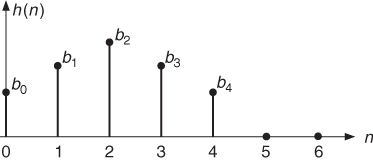
A graphical illustration of the impulse response of a five-tap FIR filter is shown in Figure 2.13. The Z-transform of the impulse response gives the transfer function
2.32 
and with ![]() the frequency response
the frequency response
2.33 ![]()
Figure 2.13 Impulse response of an FIR filter.
Filter Design
The filters already described such as LP, HP, BP and BR are also possible with FIR filter structures (see Figure 2.14). The N coefficients b0, …, bN−1 of a nonrecursive filter have to be computed by special design programs, which are discussed in all DSP text books. The N coefficients of the impulse response can be designed to yield a linear phase response, when the coefficients fulfill certain symmetry conditions. The simplest design is based on the inverse discrete-time Fourier transform of the ideal lowpass filter, which leads to the impulse response
2.34 ![]()
To improve the frequency response this impulse response can be weighted by an appropriate window function like Hamming or Blackman according to
2.35 ![]()
2.36 ![]()
If a lowpass filter is designed and an impulse response hLP(n) is derived, a frequency transformation of this lowpass filter leads to highpass, bandpass and bandreject filters (see Fig. 2.14).
Figure 2.14 Frequency transformations: LP and frequency transformations to BP and HP.
Frequency transformations are performed in the time domain by taking the lowpass impulse response hLP(n) and computing the following equations:
- LP-HP
2.37

- LP-BP
2.38

- LP-BR
2.39

Another simple FIR filter design is based on the FFT algorithm and is called frequency sampling. Its main idea is to specify the desired frequency response at discrete frequencies uniformly distributed over the frequency axis and calculate the corresponding impulse response. Design examples for audio processing with this design technique can be found in [Zöl05].
Musical Applications
If linear phase processing is required, FIR filter offer magnitude equalization without phase distortions. They allow real-time equalization by making use of the frequency sampling design procedure [Zöl05] and are attractive equalizer counterparts to IIR filters, as shown in [McG93]. A discussion of more advanced FIR filters for audio processing can be found in [Zöl05].
2.2.7 Convolution
Introduction
Convolution is a generic signal processing operation like addition or multiplication. In the realm of computer music, however, it has the particular meaning of imposing a spectral or temporal structure onto a sound. These structures are usually not defined by a set of a few parameters, such as the shape or the time response of a filter, but are given by a signal which lasts typically a few seconds or more. Although convolution has been known and used for a very long time in the signal-processing community, its significance for computer music and audio processing has grown with the availability of fast computers that allow long convolutions to be performed in a reasonable period of time.
Signal Processing
We could say in general that the convolution of two signals means filtering one with the other. There are several ways of performing this operation. The straightforward method is a direct implementation in a FIR filter structure, but it is computationally very inefficient when the impulse response is several thousand samples long. Another method, called fast convolution, makes use of the FFT algorithm to dramatically speed up the computation. The drawback of fast convolution is that it has a processing delay equal to the length of two FFT blocks, which is objectionable for real-time applications, whereas the FIR method has the advantage of providing a result immediately after the first sample has been computed. In order to take advantage of the FFT algorithm while keeping the processing delay to a minimum, low-latency convolution schemes have been developed which are suitable for real-time applications [Gar95, MT99].
The result of convolution can be interpreted in both the frequency and time domains. If a(n) and b(n) are the two convolved signals, the output spectrum will be given by the product of the two spectra S(f) = A(f) · B(f). The time interpretation derives from the fact that if b(n) is a pulse at time k, we will obtain a copy of a(n) shifted at time k0, i.e., s(n) = a(n − k). If b(n) is a sequence of pulses, we will obtain a copy of a(n) in correspondence to every pulse, i.e., a rhythmic, pitched or reverberated structure, depending on the pulse distance. If b(n) is pulse-like, we obtain the same pattern with a filtering effect. In this case b(n) should be interpreted as an impulse response. Thus convolution will result in subtractive synthesis, where the frequency shape of the filter is determined by a real sound. For example convolution with a bell sound will be heard as filtered by the resonances of the bell. In fact the bell sound is generated by a strike on the bell and can be considered as the impulse response of the bell. In this way we can simulate the effect of a sound hitting a bell, without measuring the resonances and designing the filter. If both sounds a(n) and b(n) are complex in time and frequency, the resulting sound will be blurred and will tend to lack the original sound's character. If both sounds are of long duration and each has a strong pitch and smooth attack, the result will contain both pitches and the intersection of their spectra.
Musical Applications
When a sound is convolved with the impulse responses of a room, it is projected in the corresponding virtual auditory space [DMT99]. A diffuse reverberation can be produced by convolving with broad-band noise having a sharp attack and exponentially decreasing amplitude. Another example is obtained by convolving a tuba glissando with a series of snare-drum strokes. The tuba is transformed into something like a Tibetan trumpet playing in the mountains. Each stroke of the snare drum produces a copy of the tuba sound. Since each stroke is noisy and broadband, it acts like a reverberator. The series of strokes acts like several diffusing boundaries and produces the type of echo that can be found in natural landscapes [DMT99].
The convolution can be used to map a rhythm pattern onto a sampled sound. The rhythm pattern can be defined by positioning a unit impulse at each desired time within a signal block. The convolution of the input sound with the time pattern will produce copies of the input signal at each of the unit impulses. If the unit impulse is replaced by a more complex sound, each copy will be modified in its timbre and in its time structure. If a snare drum stroke is used, the attacks will be smeared and some diffusion will be added. The convolution has an effect both in the frequency and in the time domain. Take a speech sound with sharp frequency resonances and a rhythm pattern defined by a series of snare-drum strokes. Each word will appear with the rhythm pattern and the rhythm pattern will be heard in each word with the frequency resonances of the initial speech sound.
Convolution as a tool for musical composition has been investigated by composers such as Horacio Vaggione [m-Vag96, Vag98] and Curtis Roads [Roa97]. Because convolution has a combined effect in the time and frequency domains, some expertise is necessary to foresee the result of the combination of two sounds.