9.4 Examples of Adaptive DAFX

As explained in this chapter's introduction, several effects already made use of adaptive control a long time before recent studies tended to generalize this concept to all audio effects [VA01, ABL+03]. Such effects were developed for technical or musical purposes, as answers to specific needs (e.g., auto-tune, compressor, cross-synthesis). Using the framework presented in this chapter, we can now ride on the adaptive wave, and present old and new adaptive effects in terms of: their form, the sound features that are used, the mapping of sound features to effect control parameters, the modifications of implementation techniques that are required, and the perceptual effect of the ADAFX.

9.4.1 Adaptive Effects on Loudness

Adaptive Sound-level Change

By controlling the sound level from a sound feature, we perform an amplitude modulation with a signal which is not monosinusoidal. This generalizes compressor/expander, noise gate/limiter, and cross-duking, which all are specific cases in terms of sound-feature extraction and mapping. Adaptive amplitude modulation controlled by c(n) provides the following signal

9.58

By deriving c(n) from the sound-intensity level, one obtains compressor/expander and noise gate/limiter. By using the voiciness v(n) ∈ [0, 1] and a mapping law, one obtains a ‘voiciness gate,’ which is a timbre effect that removes voicy sounds and leaves only noisy sounds (which differs from the de-esser [DZ02] that mainly removes the ‘s’). Adaptive sound-level change is also useful for attack modification of instrumental and electroacoustic sounds (differently from compressor/expander), thus modifying loudness and timbre. If using a computational model of perceived loudness, one can make a feedforward adaptive loudness change, that tries to reach a target loudness by means of iterative computations on the output loudness depending on the gain applied.

Adaptive Tremolo

A tremolo, of monosinusoidal amplitude modulation, is an effect for which either the rate (or modulation frequency fm(n)) and the depth d(n), or both, can be derived from sound features. The time-varying amplitude modulation is then expressed using a linear scale

9.59

where fS the audio sampling rate. It may also be expressed using a logarithmic scale according to

9.60

The modulation function is sinusoidal, but may be replaced by any other periodic function (e.g., triangular, exponential, logarithmic or other). The real-time implementation only requires an oscillator, a warping function, and an audio rate control. Adaptive tremolo allows for a more natural tremolo that accelerates/slows down (which also sounds like a rhythm modification) and emphasizes or de-emphasizes, depending on the sound content (which is perceived as a loudness modification). Figure 9.33 shows an example where the fundamental frequency f0(m) ∈ [780, 1420] Hz and the sound-intensity level a(m) ∈ [0, 1] are mapped to the control rate and the depth according to the following mapping rules

9.61

9.62

9.4.2 Adaptive Effects on Time

Adaptive Time-warping

Time-warping is non-linear time-scaling. This non-real-time processing uses a time-scaling ratio γ(m) that varies with m the block index. The sound is then alternatively locally time-expanded when γ(m) > 1, and locally time-compressed when γ(m) < 1. The adaptive control is provided with the input signal (feedforward adaption). The implementation can be achieved either using a constant analysis step increment RA and a time-varying synthesis step increment RS(m), or using a time-varying RA(m) and constant RS, thus providing more implementation efficiency. In the latter case, the recursive formulae of the analysis time index tA and the synthesis time index tS are given by

9.63

9.64

with the analysis step increment according to

9.65

Adaptive time-warping provides improvement to the usual time-scaling, for example by minimizing the timbre modification. It allows for time-scaling with attack preservation when using an attack/transient detector to vary the time-scaling ratio [Bon00, Pal03].

Using auto-adaptive time-warping, we can apply fine changes in duration. A first example consists of time-compressing the gaps and time-expanding the sounding parts: the time-warping ratio γ is computed from the intensity level a(n) ∈ [0, 1] using a mapping law such as , with a0 as a threshold. A second example consists of time-compressing the voicy parts and time-expanding the noisy parts of a sound, using the mapping law , with v(n) ∈ [0, 1] the voiciness and v0 the voiciness threshold. When used for local changes of duration, it provides modifications of timbre and expressiveness by modifying the attack, sustain and decay durations. Using cross-adaptive time-warping, time-folding of sound A is slowed down or sped up depending on the sound B content. Generally speaking, adaptive time-warping allows for a re-interpretation of recorded sounds, for modifications of expressiveness (music) and perceived emotion (speech). Unfortunately, there is a lack of knowledge of and investigation into the link between sound features and their mapping to the effect control on one side, and the modifications of expressiveness on the other side.

Adaptive Time-warping that Preserves Signal Length

When applying time-warping with adaptive control, the signal length is changed. To preserve the original signal length, we must evaluate the length of the time-warped signal according to the adaptive control curve. Then, a specific mapping function is applied to the time-warping ratio γ so that it verifies the synchronization constraint.

Synchronization Constraint

Time indices in Equations (9.63) and (9.64) are functions that depend on γ and m as given by

9.66

9.67

The analysis signal length differs from the synthesis signal length LS = MRS. This is no more the case for verifying the synchronization constraint

9.68

Three Synchronization Schemes

The constraint ratio can be derived from γ by:

An example is provided in Figure 9.34. Each of these modifications imposes a specific behavior on the time-warping control. For example, the exponential weighting is the only synchronization technique that preserves the locations where the signal has to be time-compressed or expanded: when γ > 1 and when γ < 1.

Synchronization that Preserves Boundaries

However, none of these three synchronization schemes ensure to preserve and , the boundaries of as given by the user. A solution consists in using the clipping function

9.72

The iterative solution that both preserves the synchronization constraint of Equation (9.68) and the initial boundaries can be derived as

9.73

where i = 1, 2, 3 respectively denotes addition, multiplication, and exponential weighting. The adaptive time-warping that preserves the signal length can be used for various things, among which expressiveness change (slight modifications of a solo improvisation that still sticks to the beat), a more natural chorus (when combined with adaptive pitch-shifting), or a swing change.

Swing Change

Adaptive time-warping that preserves the signal length provides groove change when giving several synchronization points [VZA06]. When time-scaling is controlled by an analysis from a beat tracker, synchronization points can be beat-dependent and then the swing can be changed [GFB03] by displacing one every two beats either to make them even (binary rhythm) of uneven with the rule of thumb 2/3 and 1/3 (ternary rhythm). This effect modifies time and rhythm.

Time-scaling that Preserves the Vibrato and Tremolo

Adaptive time-scaling also allows for time-scaling sounds with vibrato, for instance when combined with adaptive pitch-shifting controlled by a vibrato estimator: vibrato is removed, the sound is time-scaled, and vibrato with same frequency and depth is applied [AD98]. Using the special sinusoidal model [MR04], both vibrato (often modeled and reduced as frequency modulation) and tremolo (amplitude modulation) can be preserved by applying the resampling of control parameters on the partials of partials. This allows one to time-scale the portion of the sound which would be considered as ‘sustained,’ while leaving untouched the attack and release.

9.4.3 Adaptive Effects on Pitch

Adaptive Pitch-shifting

Using any of the techniques proposed for the usual pitch-shifting with formant preservation (PSOLA, phase vocoder combined with source-filter separation, and additive model), adaptive pitch-shifting can be performed in real time, with its pitch-shift ratio ρ(m) defined in the middle of the block as

9.74

where F0,in(m) (resp. F0,out(m)) denotes the fundamental frequency of the input (resp. the output) signal. The additive model allows for varying pitch-shift ratios, since the synthesis can be made sample by sample in the time domain [MQ86]. The pitch-shifting ratio is then interpolated sample by sample between two blocks. PSOLA allows for varying pitch-shifting ratios as long as one performs at the block level and performs energy normalization during the overlap-add technique. The phase vocoder technique has to be modified in order to permit that two overlap-added blocks have the same pitch-shifting ratio for all the samples they share, thus avoiding phase cancellation of overlap-added blocks. First, the control curve must be low pass filtered to limit the pitch-shifting ratio variations. In doing so, we can consider that the spectral envelope does not vary inside a block, and then use the source-filter decomposition to resample only the source. Second, the variable sampling rate FA(m) implies a variable length of the synthesis block NS(m) = NA/ρ(m) and so a variable energy of the overlap-added synthesis signal. The solution we chose consists in imposing a constant synthesis block size Nc = NU/max ρ(m), either by using a variable analysis block size NA(m) = ρ(m)NU and then NS = NU, or by using a constant analysis block size NA = NU and post-correcting the synthesis block xps according to

9.75

where h is the Hanning window, is the number of samples of the synthesis block m, xps(n) is the resampled and formant-corrected block n = 1, ..., N(m), w is the warped analysis window defined for n = 1, ..., N(m) as , and ρs(n) is the pitch-shifting ratio ρ(m) resampled at the signal sampling rate FA.

A musical application of adaptive pitch-shifting is adaptive detuning, obtained by adding to a signal its pitch-shifted version with a lower than a quarter-tone ratio (this also modifies timbre). For instance, adaptive detuning can be controlled by the amplitude as ρ(n) = 20.25·a(n), where louder sounds are the most detuned. Adaptive pitch-shifting allows for melody change when controlled by long-term features such as the pitch of each note of a musical sentence [GPAH03]. The auto-tune is a feedback-adaptive pitch-shifting effect, where the pitch is shifted so that the processed sound reaches a target pitch. Adaptive pitch-shifting is also useful for intonation change, as explained below.

Harmonizer

As it will be further explained in Chapter 10, a vocal chorus can be harmonized by adding pitch-shifted versions of a voice sound. These pitch-shifted versions are tuned to one given target degree in the current musical scale, so that chords of voices are obtained. This is very similar to the auto-tune (feedback-adaptive effect), except that the target pitch is not the pitch in the scale which is nearest the original pitch, but a pitch with a specific relation to the original voice pitch. This effect, combined with other effects such as auto-tune, reverberation, etc., has been widely used in recent products such as the Vocaloid by Yamaha, and the VoiceOne by TC Helicon.

Adaptive Intonation Change

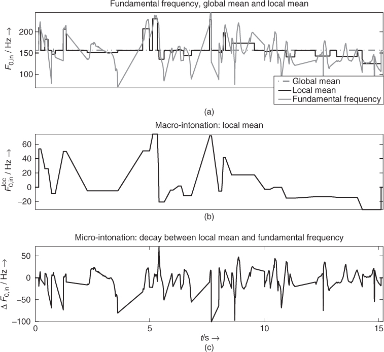
Intonation is the pitch information contained in prosody of human speech. It is composed of the macro-intonation and the micro-intonation [Cri82]. To compute these two components, the fundamental frequency F0,in(m) is segmented over time. Its local mean is the macro-intonation structure for a given segment, and the remainder is the micro-intonation structure,5 as shown in Figure 9.35. This yields the following decomposition of the input fundamental frequency

9.76

The adaptive intonation change is a non-real-time effect that modifies the fundamental frequency trends by deriving (α, β, γ) from sound features, using the decomposition

9.77

where is the mean of F0,in over the whole signal [AV03]. One can independently control the mean fundamental frequency (γ e.g., controlled by the first formant frequency), the macro-intonation structure (α e.g., controlled by the second formant frequency) and the micro-intonation structure (β e.g., controlled by the intensity level a(m)); as well as strengthen (α ≥ 1 and β ≥ 1), flatten (0 ≤ α < 1 and 0 ≤ β < 1), or inverse (α < 0 and β < 0) an intonation, thus modifying the voice ambitus, but also the whole expressiveness of speech, similarly to people from different countries speaking a foreign language with different accents.

9.4.4 Adaptive Effects on Timbre

The perceptual attribute of timbre offers the widest category of audio effects, among which voice morphing [DGR95, CLB+00] and voice conversion, spectral compressor (also known as Contrast [Fav01]), automatic vibrato (with both frequency and amplitude modulation [ABLS02]), martianization [VA02], adaptive spectral tremolo, adaptive equalizer, and adaptive spectral warping [VZA06].

Adaptive Equalizer

This effect is obtained by applying a time-varying equalizing curve Hi(m, k), which is constituted of Nq filter gains of a constant-Q filter bank. In the frequency domain, we extract a feature vector of length N denoted6 fi(m, •) from the STFT Xi(m, k) of each input channel i (the sound being mono or multi-channel). This vector feature fi(m, •) is then mapped to Hi(m, •), for example by averaging its values in each of the constant-Q segments, or by taking only the Nq first values of fi(m, •) as the gains of the filters. The equalizer output STFT is then

9.78

If Hi(m, k) varies too rapidly, the perceived effect is not varying equalizer/filtering, but ring modulation of partials, and potentially phasing. To avoid this, we low pass filter Hi( • , k) in time [VD04], with L the down sampling ratio, FI = FB/L the equalizer control sampling rate, and FB the block sampling rate. This is obtained by linear interpolation between two key vectors denoted CP−1 and CP (see Figure 9.36). For each block position m, PL ≤ m ≤ (P + 1)L, the vector feature fi(m, •) is given by

9.79

with α(m) = (m − PL)/L the interpolation ratio. Real-time implementation requires the extraction of a fast-computing key vector CP(m, k), such as the samples buffer , or the spectral envelope CP(m, k) = E(PL, k). However, non-real-time implementations allow for using more computationally expensive features, such as a harmonic comb filter, thus providing an odd/even harmonics balance modification.

Adaptive Spectral Warping

Harmonicity is adaptively modified when using spectral warping with an adaptive warping function W(m, k). The STFT magnitude is computed by

9.80

The warping function is given by

9.81

and varies in time according to two control parameters: a vector C2(m, k) ∈ [1, N], k = 1, ..., N (e.g., the spectral envelope E or its cumulative sum) which is the maximum warping function, and an interpolation ratio C1(m) ∈ [0, 1] (e.g., the energy, the voiciness), which determines the warping depth. An example is shown in Figure 9.37, with C2(m, k) derived from the spectral envelope E(m, k) as

9.82

This mapping provides a monotonous curve, and prevents the spectrum folding over. Adaptive spectral warping allows for dynamically changing the harmonicity of a sound. When applied only to the source, it allows for better in-harmonizing of voice or a musical instrument since formants are preserved.

9.4.5 Adaptive Effects on Spatial Perception

Adaptive Panning

Usually, panning requires the use of both a modification of left and right intensity levels and delays. In order to avoid the Doppler effect, delays are not taken into account in this example. With adaptive control, the azimuth angle varies in time according to sound features. A constant power panning with the Blumlein law [Bla83] gives the following gains

9.83

9.84

A sinusoidal control θ(n) = sin(2πfpann/FA) with fpan > 20 Hz is not heard anymore as a motion, but as a ring modulation (with a phase decay of π/2 between the two channels). With more complex motions obtained from sound feature control, this effect does not appear because the motion is not sinusoidal and varies most of the time under 20 Hz. The fast motions cause a stream segregation effect [Bre90], and the coherence in time between the sound motion and the sound content gives the illusion of splitting a monophonic sound into several sources. An example consists of panning synthetic trumpet sounds (obtained by frequency-modulation techniques [Cho71]) with an adaptive control derived from brightness, which is a strong perceptual indicator of brass timbre [Ris65], given by

9.85

Low-brightness sounds are left panned, whereas high brightness sounds are right panned. Brightness of trumpet sounds evolves differently during notes, attack and decay, implying that the sound attack moves fast from left to right, whereas the sound decay moves slowly from right to left. This adaptive control then provides a spatial spreading effect.

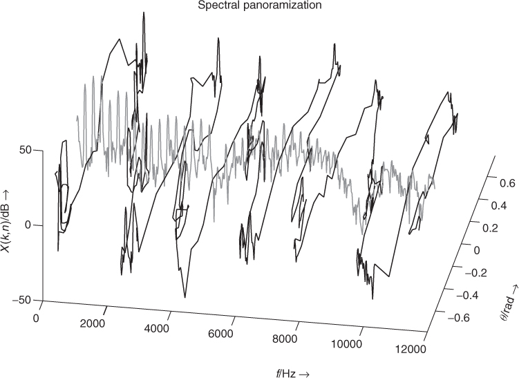
Adaptive Spectral Panning

Panning in the spectral domain allows for intensity panning by modifying the left and right spectrum magnitudes as well as for time delays by modifying the left and right spectrum phases. Using the phase vocoder, we only use intensity panning in order to avoid the Doppler effect, thus requiring slow motions of sound. To each frequency bin of the input STFT X(m, k) we attribute a position given by the panning angle θ(m, k) derived from sound features. The resulting gains for left and right channels are then

9.86

9.87

In this way, each frequency bin of the input STFT is panned separately from its neighbors (see Figure 9.38): the original spectrum is then split across the space between two loudspeakers. To avoid a phasiness effect due to the lack of continuity of the control curve between neighboring frequency bins, a smooth control curve is needed, such as the spectral envelope. In order to control the variation speed of the spectral panning, θ(m, k) is computed from a time-interpolated value of a control vector (see the adaptive equalizer, Section 9.4.4). This effect adds envelopment to the sound when the panning curve is smoothed. Otherwise, the signal is split into virtual sources having more or less independent motions and speeds. In the case the panning vector θ(m, •) is derived from the magnitude spectrum with a multi-pitch tracking technique, it allows for source separation. When derived from the voiciness v(m) as , the sound localization varies between a point during attacks and a wide spatial spread during steady state, simulating width variations of the sound source.

Spatialization

Both adaptive panning and adaptive spectral panning can be extended to 3-D sound projection, using techniques such as VBAP techniques, and so on. For instance, the user defines a trajectory (for example an ellipse), onto which the sound moves, with adaptive control on the position, the speed, or the acceleration. Concerning the position control, the azimuth can depend on the chroma , splitting the sounds into a spatial chromatic scale. The speed control adaptively depending on voiciness as allows for the sound to move only during attacks and silences; conversely, an adaptive control of speed given as allows for the sound to move only during steady states, and not during attacks and silences.

9.4.6 Multi-dimensional Adaptive Effects

Various adaptive effects affect several perceptual attributes simultaneously: adaptive resampling modifies time, pitch and timbre; adaptive ring modulation modifies only harmonicity when combined to formant preservation, and harmonicity and timbre when combined with formants modifications [VD04]; gender change combines pitch-shifting and adaptive formant-shifting [ABLS01, ABLS02] to transform a female voice into a male voice, and vice versa. We now present two other multi-dimensional adaptive effects: adaptive robotization, which modifies pitch and timbre, and adaptive granular delay, which modifies spatial perception and timbre.

Adaptive Robotization

Adaptive robotization changes expressiveness on two perceptual attributes, namely intonation (pitch) and roughness (timbre), and allows the transformation a human voice into an expressive robot voice [VA01]. This consists of zeroing the phase φ(m, k) of the grain STFT X(m, k) at a time index given by sound features: Y(m, k) = |X(m, k)|, and zeroing the signal between two blocks [VA01, AKZ02b]. The synthesis time index tS(m) = tA(m) is recursively given as

9.88

The step increment is also the period of the robot voice, i.e., the inverse of the robot fundamental frequency to which sound features are mapped (e.g., the spectral centroid as F0(m) = 0.01 · cgs(m), in Figure 9.39). Its real-time implementation implies the careful use of a circular buffer, in order to allow for varying window and step increments. Both the harmonic and the noisy part of the sound are processed, and formants are locally preserved for each block. However, the energy of the signal is not preserved, due to the zero-phasing, the varying step increment, and the zeroing process between two blocks, resulting in a pitch and modifying the loudness of noisy content. An annoying buzz sound is then perceived, and can be easily removed by reducing the loudness modification. After zeroing the phases, the synthesis grain is multiplied by the ratio of analysis to synthesis intensity level computed on the current block m given by

9.89

A second adaptive control is given by the block size N(m) and allows for changing the robot roughness: the lower the block length, the higher the roughness. At the same time, it allows preservation of the original pitch (e.g., N ≥ 1024) or removal (e.g., N ≤ 256), with an ambiguity in between. This is due to the fact that zero phasing a small block creates a main peak in the middle of the block and implies amplitude modulation (and then roughness). Inversely, zero phasing a large block creates several additional peaks in the window, the periodicity of the equally spaced secondary peaks being responsible for the original pitch.

Adaptive Granular Delay

This effect consists of applying delays to sound grains, with constant grain size N and step increment RA [VA01], and varying delay gain g(m) and/or delay time τ(m) derived from sound features (see Figure 9.40). In non-real-time applications, any delay time is possible, even fractional delay times [LVKL96], since each grain repetition is overlapped and added into a buffer. However, real-time implementations require limiting the number of delay lines, and so forth, to quantize delay time and delay gain control curves to a limited number of values. In our experience, 10 values for the delay gain and 30 for the delay time is a good minimum configuration, yielding 300 delay lines.

In the case where only g(m) varies, the effect is a combination between delay and timbre morphing (spatial perception and timbre). For example, when applying this effect to a plucked string sound and controlling the gain with a voiciness feature as , the attacks are repeated a much longer time than the sustain part. With the complementary mapping , the attacks rapidly disappear from the delayed version, whereas the sustain part is still repeated.

In the case where only τ(m) varies, the effect is a kind of granular synthesis with adaptive control, where grains collapse in time, thus implying modifications of time, timbre, and loudness. With a delay time derived from voiciness τ(m) = v(m) (in seconds), attack and sustain parts of a plucked string sound have different delay times, so sustain parts may be repeated before the attack with repetitions going on, as depicted Figure 9.40: not only are time and timbre are modified, but also loudness, since the grain superposition is uneven.

Adaptive granular delay is a perfect example of how the creative modification of an effect with adaptive control offers new sound transformation possibilities. It also shows how the frontiers between the perceptual attributes modified by the effect may be blurred.

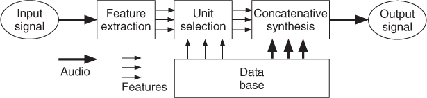
9.4.7 Concatenative Synthesis

The concept of concatenative synthesis is already in use for speech synthesis. An overview of this technique for audio processing can be found in [Sch07]. From an audio effects point of view it is an adaptive audio effect, which is controlled by low-level and high-level features extracted from the incoming audio signal and then uses sound snippets from a database to resynthesize a similar input audio. Figure 9.41 shows the functional units of such a signal-processing scheme. Sound features are derived from a block-by-block analysis scheme, which are then used for the selection of sound units from a sound database which possess similar sound features. These selected sound units are then used in a concatenative synthesis to reconstruct an audio signal. The concatenative synthesis can be performed by all time- and frequency-domain techniques discussed inside the DAFx book. The following M-file 9.15 shows the main processing steps for a concatenative singing resynthesis used in [FF10]. The script only presents the minimum number of features for singing resynthesis. It extracts energy, pitch, and LPC frequency response (no pitch smoothing or complex phonetic information) and searches for the best audio frame with a similar pitch. It uses the chosen frame, changes its gain to get a similar energy, and adds it to the output (no phase alignment or pitch changing). Further improvements and refinements are introduced in [FF10].