
In this section we introduce a set of effects and transformations that can be added to some of the analysis-synthesis frameworks that have just been presented. To do that we first need to change a few things on the implementations given above in order to make them suitable for incorporating the code for the transformations. We have to add new variables to handle the synthesis data and for controlling effects. Other modifications in the code are related to peak continuation and phase propagation. We first focus on the sinusoidal plus residual model, and next we will use the harmonic-based model.
10.4.1 Sinusoidal Plus Residual
In the implementation of the sinusoidal plus residual model presented, now we use different variables for analysis and synthesis parameters and keep a history of the last frame values. This is required for continuing analysis spectral peaks and propagating synthesis phases. The peak continuation implementation is really simple: each current frame peak is connected to the closest peak in frequency of the last frame. The phase propagation is also straightforward: it assumes that the frequency of connected peaks evolves linearly between consecutive frames. Note that when computing the residual we have to be careful to subtract the analysis sinusoids (not the synthesis ones) to the input signal. Another significant change is that here we use the parameter maxnS to limit the number of sinusoids. With that restriction, peaks found are sorted by energy and only the first maxnS are taken into account.
M-file 10.14 (spsmodel.m)
function [y,yh,ys] = spsmodel(x,fs,w,N,t,maxnS,stocf)
% Authors: J. Bonada, X. Serra, X. Amatriain, A. Loscos
% Analysis/synthesis of a sound using the sinusoidal harmonic model
% x: input sound, fs: sampling rate, w: analysis window (odd size),
% N: FFT size (minimum 512), t: threshold in negative dB,
% maxnS: maximum number of sinusoids,
% stocf: decimation factor of mag spectrum for stochastic analysis
% y: output sound, yh: harmonic component, ys: stochastic component
M = length(w); % analysis window size
Ns = 1024; % FFT size for synthesis
H = 256; % hop size for analysis and synthesis
N2 = N/2+1; % half-size of spectrum
soundlength = length(x); % length of input sound array
hNs = Ns/2; % half synthesis window size
hM = (M-1)/2; % half analysis window size
pin = max(hNs+1,1+hM); % initialize sound pointer to middle of analysis window
pend = soundlength-max(hM,hNs); % last sample to start a frame
fftbuffer = zeros(N,1); % initialize buffer for FFT
yh = zeros(soundlength+Ns/2,1); % output sine component
ys = zeros(soundlength+Ns/2,1); % output residual component
w = w/sum(w); % normalize analysis window
sw = zeros(Ns,1);
ow = triang(2*H-1); % overlapping window
ovidx = Ns/2+1-H+1:Ns/2+H; % overlap indexes
sw(ovidx) = ow(1:2*H-1);
bh = blackmanharris(Ns); % synthesis window
bh = bh ./ sum(bh); % normalize synthesis window
wr = bh; % window for residual
sw(ovidx) = sw(ovidx) ./ bh(ovidx);
sws = H*hanning(Ns)/2; % synthesis window for stochastic
lastysloc = zeros(maxnS,1); % initialize synthesis harmonic locations
ysphase = 2*pi*rand(maxnS,1); % initialize synthesis harmonic phases
fridx = 0;
while pin<pend
%-----analysis-----%
xw = x(pin-hM:pin+hM).*w(1:M); % window the input sound
fftbuffer = fftbuffer*0; % reset buffer;
fftbuffer(1:(M+1)/2) = xw((M+1)/2:M); % zero-phase window in fftbuffer
fftbuffer(N-(M-1)/2+1:N) = xw(1:(M-1)/2);
X = fft(fftbuffer); % compute the FFT
mX = 20*log10(abs(X(1:N2))); % magnitude spectrum
pX = unwrap(angle(X(1:N/2+1))); % unwrapped phase spectrum
ploc = 1 + find((mX(2:N2-1)>t) .* (mX(2:N2-1)>mX(3:N2)) ...
.* (mX(2:N2-1)>mX(1:N2-2))); % find peaks
[ploc,pmag,pphase] = peakinterp(mX,pX,ploc); % refine peak values
% sort by magnitude
[smag,I] = sort(pmag(:),1,'descend'),
nS = min(maxnS,length(find(smag>t)));
sloc = ploc(I(1:nS));
sphase = pphase(I(1:nS));
if (fridx==0)
% update last frame data for first frame
lastnS = nS;
lastsloc = sloc;
lastsmag = smag;
lastsphase = sphase;
end
% connect sinusoids to last frame lnS (lastsloc,lastsphase,lastsmag)
sloc(1:nS) = (sloc(1:nS)∼=0).*((sloc(1:nS)-1)*Ns/N); % synth. locs
lastidx = zeros(1,nS);
for i=1:nS
[dev,idx] = min(abs(sloc(i) - lastsloc(1:lastnS)));
lastidx(i) = idx;
end
ri= pin-hNs; % input sound pointer for residual analysis
xr = x(ri:ri+Ns-1).*wr(1:Ns); % window the input sound
Xr = fft(fftshift(xr)); % compute FFT for residual analysis
Xh = genspecsines(sloc,smag,sphase,Ns); % generate sines
Xr = Xr-Xh; % get the residual complex spectrum
mXr = 20*log10(abs(Xr(1:Ns/2+1))); % magnitude spectrum of residual
mXsenv = decimate(max(-200,mXr),stocf); % decimate the magnitude spectrum
% and avoid -Inf
%-----synthesis data-----%
ysloc = sloc; % synthesis locations
ysmag = smag(1:nS); % synthesis magnitudes
mYsenv = mXsenv; % synthesis residual envelope
%-----transformations-----%
%-----synthesis-----%
if (fridx==0)
lastysphase = ysphase;
end
if (nS>lastnS)
lastysphase = [ lastysphase ; zeros(nS-lastnS,1) ];
lastysloc = [ lastysloc ; zeros(nS-lastnS,1) ];
end
ysphase = lastysphase(lastidx(1:nS)) + 2*pi*( ...
lastysloc(lastidx(1:nS))+ysloc)/2/Ns*H; % propagate phases
lastysloc = ysloc;
lastysphase = ysphase;
lastnS = nS; % update last frame data
lastsloc = sloc; % update last frame data
lastsmag = smag; % update last frame data
lastsphase = sphase; % update last frame data
Yh = genspecsines(ysloc,ysmag,ysphase,Ns); % generate sines
mYs = interp(mYsenv,stocf); % interpolate to original size
roffset = ceil(stocf/2)-1; % interpolated array offset
mYs = [ mYs(1)*ones(roffset,1); mYs(1:Ns/2+1-roffset) ];
mYs = 10.∧(mYs/20); % dB to linear magnitude
pYs = 2*pi*rand(Ns/2+1,1); % generate phase spectrum with random values
mYs1 = [mYs(1:Ns/2+1); mYs(Ns/2:-1:2)]; % create complete magnitude spectrum
pYs1 = [pYs(1:Ns/2+1); -1*pYs(Ns/2:-1:2)]; % create complete phase spectrum
Ys = mYs1.*cos(pYs1)+1i*mYs1.*sin(pYs1); % compute complex spectrum
yhw = fftshift(real(ifft(Yh))); % sines in time domain using inverse FFT
ysw = fftshift(real(ifft(Ys))); % stochastic in time domain using IFFT
yh(ri:ri+Ns-1) = yh(ri:ri+Ns-1)+yhw(1:Ns).*sw; % overlap-add for sines
ys(ri:ri+Ns-1) = ys(ri:ri+Ns-1)+ysw(1:Ns).*sws; % overlap-add for stochastic
pin = pin+H; % advance the sound pointer
fridx = fridx+1;
end
y= yh+ys; % sum sines and stochastic
Now we have an implementation of the sinusoidal plus residual model ready to be used for sound transformations. In order to use the different effects we just have to add the code of the effect after the line %-----transformations-----%.
Filtering
Filters are probably the paradigm of a classical effect. In our implementation of filtering we take advantage of the sinusoidal plus residual model, which allows us to modify the amplitude of any partial present in the sinusoidal component.
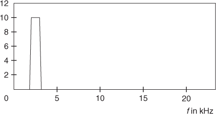
For example, we can implement a band pass filter defined by (x, y) points where x is the frequency value in Hertzs and y is the amplitude factor to apply (see Figure 10.19). In the example code given below, we define a band pass filter which supreses sinusoidal frequencies not included in the range [2100 3000].
M-file 10.15 (spsfiltering.m)
% Authors: J. Bonada, X. Serra, X. Amatriain, A. Loscos
%----- filtering -----%
Filter=[ 0 2099 2100 3000 3001 fs/2; % Hz
-200 -200 0 0 -200 -200 ]; % db
ysmag = ysmag+interp1(Filter(1,:),Filter(2,:),ysloc/Ns*fs);
Figure 10.19 Bandpass filter with arbitrary resolution.
Frequency Shifting
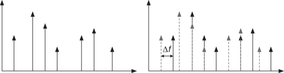
In this example we introduce a frequency shift factor to all the partials of our sound (see Figure 10.20). Note, though, that if the input sound is harmonic, then adding a constant to every partial produces a sound that will be inharmonic.
M-file 10.16 (spsfrequencyshifting.m)
% Authors: J. Bonada, X. Serra, X. Amatriain, A. Loscos
%-----frequency shift-----%
fshift = 100;
ysloc = (ysloc>0).*(ysloc + fshift/fs*Ns); % frequency shift in Hz
Figure 10.20 Frequency shift of the partials.
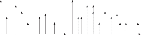
Frequency Stretching
Another effect we can implement following this same idea is to add a stretching factor to the frequency of every partial. The relative shift of every partial will depend on its original partial index, following the formula:
10.17 ![]()
Figure 10.21 illustrates this frequency stretching.
Figure 10.21 Frequency stretching.
M-file 10.17 (spsfrequencystretching.m)
%Authors: J. Bonada, X. Serra, X. Amatriain, A. Loscos
%-----frequency stretch-----%
fstretch = 1.1;
ysloc = ysloc .* (fstretch.∧[0:length(ysloc)-1]'),
Frequency Scaling
In the same way, we can scale all the partials multiplying them by a given scaling factor. Note that this effect will act as a pitch shifter without timbre preservation.
M-file 10.18 (spsfrequencyscaling.m)
% Authors: J. Bonada, X. Serra, X. Amatriain, A. Loscos
%-----frequency scale-----%
fscale = 1.2;
ysloc = ysloc*fscale;
Time Scaling
Time scaling is trickier and we have to modify some aspects of the main processing loop. We now use two different variables for the input and output times (pin and pout). The idea is that the analysis hop size will not be constant, but will depend on the time-scaling factor, while the synthesis hop size will be fixed. If the sound is played slower (time expansion), then the analysis hop size will be smaller and pin will be incremented by a smaller amount. Otherwise, when the sound is played faster (time compression), the hop size will be larger. Instead of using a constant time-scaling factor, here we opt for a more flexible approach by setting a mapping between input and output time. This allows, for instance, easy alignment of two audio signals by using synchronization onset times as the mapping function.
The following code sets the input/output time mapping. It has to be added at the beginning of the function. In this example, the sound is time expanded by a factor of 2.
M-file 10.19 (spstimemappingparams.m)
% Authors: J. Bonada, X. Serra, X. Amatriain, A. Loscos
%-----time mapping-----%
timemapping = [ 0 1; % input time (sec)
0 2 ]; % output time (sec)
timemapping = timemapping *soundlength/fs;
outsoundlength = 1+round(timemapping(2,end)*fs); % length of output sound
Since the output and input durations may be different, we have to change the creation of the output signal variables so that they match the output duration.
M-file 10.20 (spstimemappinginit.m)
% Authors: J. Bonada, X. Serra, X. Amatriain, A. Loscos
yh = zeros(outsoundlength+Ns/2,1); % output sine component
ys = zeros(outsoundlength+Ns/2,1); % output residual component
Finally, we modify the processing loop. Note the changes in the last part, where the synthesis frame is added to the output vectors yh and ys. Note also that pin is computed from the synthesis time pout by interpolating the time-mapping function.
M-file 10.21 (spstimemappingprocess.m)
% Authors: J. Bonada, X. Serra, X. Amatriain, A. Loscos
poutend = outsoundlength-hNs; % last sample to start a frame
pout = pin;
minpin = 1+max(hNs,hM);
maxpin = min(length(x)-max(hNs,hM)-1);
fridx = 0;
while pout<poutend
pin = round( interp1(TM(2,:),TM(1,:),pout/fs,'linear','extrap') * fs );
pin = max(minpin,pin);
pin = min(maxpin,pin);
%-----analysis-----%
(...)
ro = pout-hNs; % output sound pointer for overlap
yh(ro:ro+Ns-1) = yh(ro:ro+Ns-1)+yhw(1:Ns).*sw; % overlap-add for sines
ys(ro:ro+Ns-1) = ys(ro:ro+Ns-1)+ysw(1:Ns).*sws; % overlap-add for stochastic
pout = pout+H; % advance the sound pointer
fridx = fridx+1;
end
y= yh+ys; % sum sines and stochastic
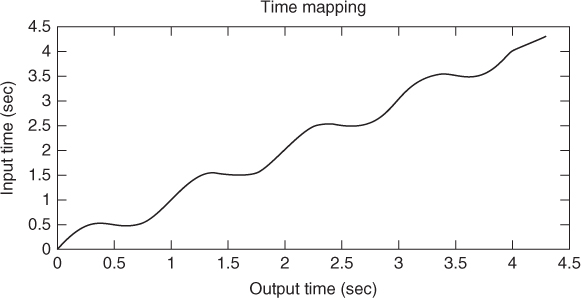
With the proposed time-mapping control we can play the input sound in forward or reverse directions at any speed, or even freeze it. The following mapping uses a sinusoidal function to combine all these possibilities (see Figure 10.22). When applied to the fairytale.wav audio example, it produces a really funny result.
M-file 10.22 (spstimemappingcomplex.m)
% Authors: J. Bonada, X. Serra, X. Amatriain, A. Loscos
tm = 0.01:0.01:.93;
timemapping = [ 0 tm+0.05*sin(8.6*pi*tm) 1 ; % input time --> keep end value
0 tm 1 ]; % output time
timemapping = timemapping*length(x)/fs;
Figure 10.22 Complex time mapping.
10.4.2 Harmonic Plus Residual
We will now use the harmonic plus residual model and also modify the implementation above. We use different variables for analysis and synthesis parameters and we keep a history of the last frame values. As before, phase propagation is implemented assuming linear frequency evolution of harmonics. Peak continuation, however, works differently: we just connect the closest peaks to each predicted harmonic frequency. In addition, we add the modifications required to able to perform time scaling. When we apply effects to harmonic sounds, sometimes we perceive the output harmonic and residual components to be somehow unrelated, in a way that loses part of the cohesion found in the original sound. Applying a comb filter to the residual determined by the synthesis fundamental frequency helps to merge both components and perceive them as a single entity. We have added such filter to the code below. Note also that the Yin algorithm is used by default when computing the fundamental frequency.
On the other hand, we can go a step further by implementing several transformations in the same code, and adding the corresponding control parameters as function arguments. This has the advantage that we can easily combine transformations to achieve more complex effects. Moreover, as we will see, this is great for generating several outputs with different effects to be concatenated or played simultaneously.
M-file 10.23 (hpsmodelparams.m)
function [y,yh,ys] = hpsmodelparams(x,fs,w,N,t,nH,minf0,maxf0,f0et,...
maxhd,stocf,timemapping)
% Authors: J. Bonada, X. Serra, X. Amatriain, A. Loscos
% Analysis/synthesis of a sound using the sinusoidal harmonic model
% x: input sound, fs: sampling rate, w: analysis window (odd size),
% N: FFT size (minimum 512), t: threshold in negative dB,
% nH: maximum number of harmonics, minf0: minimum f0 frequency in Hz,
% maxf0: maximim f0 frequency in Hz,
% f0et: error threshold in the f0 detection (ex: 5),
% maxhd: max. relative deviation in harmonic detection (ex: .2)
% stocf: decimation factor of mag spectrum for stochastic analysis
% timemapping: mapping between input and output time (sec)
% y: output sound, yh: harmonic component, ys: stochastic component
if length(timemapping)==0 % argument not specified
timemapping =[ 0 length(x)/fs; % input time
0 length(x)/fs ]; % output time
end
M = length(w); % analysis window size
Ns = 1024; % FFT size for synthesis
H = 256; % hop size for analysis and synthesis
N2 = N/2+1; % half-size of spectrum
hNs = Ns/2; % half synthesis window size
hM = (M-1)/2; % half analysis window size
fftbuffer = zeros(N,1); % initialize buffer for FFT
outsoundlength = 1+round(timemapping(2,end)*fs); % length of output sound
yh = zeros(outsoundlength+Ns/2,1); % output sine component
ys = zeros(outsoundlength+Ns/2,1); % output residual component
w = w/sum(w); % normalize analysis window
sw = zeros(Ns,1);
ow = triang(2*H-1); % overlapping window
ovidx = Ns/2+1-H+1:Ns/2+H; % overlap indexes
sw(ovidx) = ow(1:2*H-1);
bh = blackmanharris(Ns); % synthesis window
bh = bh ./ sum(bh); % normalize synthesis window
wr = bh; % window for residual
sw(ovidx) = sw(ovidx) ./ bh(ovidx);
sws = H*hanning(Ns)/2; % synthesis window for stochastic
lastyhloc = zeros(nH,1); % initialize synthesis harmonic locations
yhphase = 2*pi*rand(nH,1); % initialize synthesis harmonic phases
poutend = outsoundlength-max(hM,H); % last sample to start a frame
pout = 1+max(hNs,hM); % initialize sound pointer to middle of analysis window
minpin = 1+max(hNs,hM);
maxpin = min(length(x)-max(hNs,hM)-1);
while pout<poutend
pin = round( interp1(timemapping(2,:),timemapping(1,:),pout/fs,'linear',...
'extrap') * fs );
pin = max(minpin,pin);
pin = min(maxpin,pin);
%-----analysis-----%
xw = x(pin-hM:pin+hM).*w(1:M); % window the input sound
fftbuffer(:) = 0; % reset buffer
fftbuffer(1:(M+1)/2) = xw((M+1)/2:M); % zero-phase window in fftbuffer
fftbuffer(N-(M-1)/2+1:N) = xw(1:(M-1)/2);
X = fft(fftbuffer); % compute the FFT
mX = 20*log10(abs(X(1:N2))); % magnitude spectrum
pX = unwrap(angle(X(1:N/2+1))); % unwrapped phase spectrum
ploc = 1 + find((mX(2:N2-1)>t) .* (mX(2:N2-1)>mX(3:N2)) ...
.* (mX(2:N2-1)>mX(1:N2-2))); % find peaks
[ploc,pmag,pphase] = peakinterp(mX,pX,ploc); % refine peak values
yinws = round(fs*0.0125); % using approx. a 12.5 ms window for yin
yinws = yinws+mod(yinws,2); % make it even
yb = pin-yinws/2;
ye = pin+yinws/2+yinws;
if (yb<1 || ye>length(x)) % out of boundaries
f0 = 0;
else
f0 = f0detectionyin(x(yb:ye),fs,yinws,minf0,maxf0); % compute f0
end
hloc = zeros(nH,1); % initialize harmonic locations
hmag = zeros(nH,1)-100; % initialize harmonic magnitudes
hphase = zeros(nH,1); % initialize harmonic phases
hf = (f0>0).*(f0.*(1:nH)); % initialize harmonic frequencies
hi = 1; % initialize harmonic index
npeaks = length(ploc); % number of peaks found
while (f0>0 && hi<=nH && hf(hi)<fs/2) % find harmonic peaks
[dev,pei] = min(abs((ploc(1:npeaks)-1)/N*fs-hf(hi))); % closest peak
if ((hi==1 || ∼any(hloc(1:hi-1)==ploc(pei))) && dev<maxhd*hf(hi))
hloc(hi) = ploc(pei); % harmonic locations
hmag(hi) = pmag(pei); % harmonic magnitudes
hphase(hi) = pphase(pei); % harmonic phases
end
hi = hi+1; % increase harmonic index
end
hloc(1:hi-1) = (hloc(1:hi-1)∼=0).*((hloc(1:hi-1)-1)*Ns/N); % synth. locs
ri= pin-hNs; % input sound pointer for residual analysis
xr = x(ri:ri+Ns-1).*wr(1:Ns); % window the input sound
Xr = fft(fftshift(xr)); % compute FFT for residual analysis
Xh = genspecsines(hloc(1:hi-1),hmag,hphase,Ns); % generate sines
Xr = Xr-Xh; % get the residual complex spectrum
mXr = 20*log10(abs(Xr(1:Ns/2+1))); % magnitude spectrum of residual
mXsenv = decimate(max(-200,mXr),stocf); % decimate the magnitude spectrum
% and avoid -Inf
%-----synthesis data-----%
yhloc = hloc; % synthesis harmonics locs
yhmag = hmag; % synthesis harmonic amplitudes
mYsenv = mXsenv; % synthesis residual envelope
yf0 = f0; % synthesis f0
%-----transformations-----%
%-----synthesis-----%
yhphase = yhphase + 2*pi*(lastyhloc+yhloc)/2/Ns*H; % propagate phases
lastyhloc = yhloc;
Yh = genspecsines(yhloc,yhmag,yhphase,Ns); % generate sines
mYs = interp(mYsenv,stocf); % interpolate to original size
roffset = ceil(stocf/2)-1; % interpolated array offset
mYs = [ mYs(1)*ones(roffset,1); mYs(1:Ns/2+1-roffset) ];
mYs = 10.∧(mYs/20); % dB to linear magnitude
if (f0>0)
mYs = mYs .* cos(pi*[0:Ns/2]'/Ns*fs/yf0).∧2; % filter residual
end
fc = 1+round(500/fs*Ns); % 500 Hz
mYs(1:fc) = mYs(1:fc) .* ([0:fc-1]'/(fc-1)).∧2; % HPF
pYs = 2*pi*rand(Ns/2+1,1); % generate phase spectrum with random values
mYs1 = [mYs(1:Ns/2+1); mYs(Ns/2:-1:2)]; % create complete magnitude spectrum
pYs1 = [pYs(1:Ns/2+1); -1*pYs(Ns/2:-1:2)]; % create complete phase spectrum
Ys = mYs1.*cos(pYs1)+1i*mYs1.*sin(pYs1); % compute complex spectrum
yhw = fftshift(real(ifft(Yh))); % sines in time domain using IFFT
ysw = fftshift(real(ifft(Ys))); % stochastic in time domain using IFFT
ro= pout-hNs; % output sound pointer for overlap
yh(ro:ro+Ns-1) = yh(ro:ro+Ns-1)+yhw(1:Ns).*sw; % overlap-add for sines
ys(ro:ro+Ns-1) = ys(ro:ro+Ns-1)+ysw(1:Ns).*sws; % overlap-add for stochastic
pout = pout+H; % advance the sound pointer
end
y= yh+ys; % sum sines and stochastic
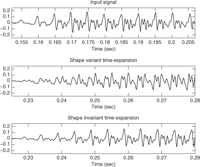
In the previous code the phase of each partial is propagated independently using the estimated frequencies. This has two disadvantages: (a) inaccuracies in frequency estimation add errors to the phase propagation that are accumulated over time; (b) the phase information of the input signal is not used, so its phase behavior will not be transferred to the output signal. In many cases, this results not only in a loss of presence and definition, often referred to as phasiness, but also makes the synthetic signal to sound artificial, especially at low pitches and transitions. This issue is very much related to the concept of shape invariance, which we introduce next.
Although we focus the following discussion on the human voice, it can be generalized to many musical instruments and sound-production systems. In a simplified model of voice production, a train of impulses at the pitch rate excites a resonant filter (i.e., the vocal tract). According to this model, a speaker or singer changes the pitch of his voice by modifying the rate at which those impulses occur. An interesting observation is that the shape of the time-domain waveform signal around the impulse onsets is roughly independent of the pitch, but it depends mostly on the impulse response of the vocal tract. This characteristic is called shape invariance. In terms of frequency domain, this shape is related to the amplitude, frequency and phase values of the harmonics at the impulse onset times. A given processing technique will be shape invariant if it preserves the phase coherence between the various harmonics at estimated pulse onsets. Figure 10.23 compares the results of a time-scaling transformation using shape-variant and -invariant methods.
Figure 10.23 Shape-variant and -invariant transformations. In this example the input signal is time-expanded by a factor of 1.5.
Several algorithms have been proposed in the literature regarding the harmonic phase-coherence for both phase-vocoder and sinusoidal modeling (for example [DiF98, Lar03]). Most of them are based on the idea of defining pitch-synchronous input and output onset times and reproducing at the output onset times the phase relationship existing in the original signal at the input onset times. Nevertheless, in order to obtain the best sound quality, it is desirable that for speech signals those detected onsets match the actual glottal pulse onsets [Bon08].
The following code uses this idea to implement a shape-invariant transformation. It should be inserted in the previous code after the line where synthesis phases are propagated, just at the beginning of the %-----synthesis-----% section.
M-file 10.24 (shapeinvariance.m)
% Authors: J. Bonada, X. Serra, X. Amatriain, A. Loscos
% shape invariance:
% assume pulse onsets to match zero phase of the fundamental
% and ideal harmonic distribution
pos = mod(hphase(1),2*pi)/2/pi; % input normalized period position
ypos = mod(yhphase(1),2*pi)/2/pi; % output normalized period position
yhphase = hphase + (ypos-pos)*2*pi*[1:length(yhloc)]';
Harmonic Filtering
As shown, a filter does not need to be characterized by a traditional transfer function, but a more complex filter can be defined. For example, the following code filters out the even partials of the input sound. If applied to a sound with a broadband spectrum, like a vocal sound, it will convert it to a clarinet-like sound.
M-file 10.25 (hpsmodelharmfiltering.m)
% Authors: J. Bonada, X. Serra, X. Amatriain, A. Loscos
%-----voice to clarinet-----%
yhloc(2:2:end)=0; % set to zero the frequency of even harmonics
% so that they won't be synthesized
Pitch Discretization
An interesting effect can be accomplished by forcing the pitch to take the nearest frequency value of the temperate scale. It is indeed a very particular case of pitch transposition, where the pitch is quantified to one of the 12 semitones into which an octave is divided. This effect is widely used on vocal sounds for dance music and is many times referred to with the misleading name of the vocoder effect.
M-file 10.26 (hpsmodelpitchdisc.m)
% Authors: J. Bonada, X. Serra, X. Amatriain, A. Loscos
%-----pitch discretization to temperate scale-----%
if (f0>0) % it has harmonics
nst = round(12*log2(f0/55)); % closest semitone
discpitch = 55*2∧(nst/12); % discretized pitch
fscale = discpitch/f0 ; % pitch transposition factor
yf0 = f0*fscale; % synthesis f0
yhloc = yhloc*fscale;
end
Pitch Transposition with Timbre Preservation
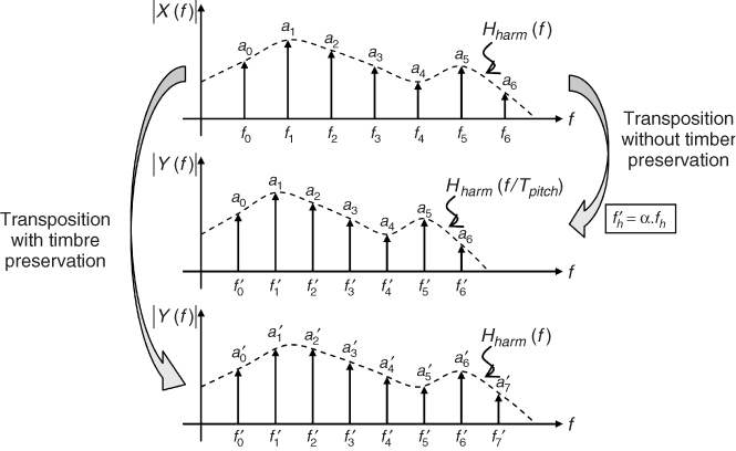
Pitch transposition is the scaling of all the partials of a sound by the same multiplying factor. An undesirable effect is obtained if the amplitude of partials is not modified. In that case, the timbre is scaled as well, producing the typical Mickey Mouse effect. This undesired effect can be avoided using the analysis harmonic spectral envelope, which is obtained from the interpolation of the harmonic amplitude values. Then, when synthesizing, we compute harmonic amplitudes interpolating this same envelope at their scaled frequency position. This is illustrated in Figure 10.24, where α is the frequency scaling factor, and Hharm the harmonic spectral envelope.
M-file 10.27 (transpositionpreservingtimbre.m)
% Authors: J. Bonada, X. Serra, X. Amatriain, A. Loscos
%-----pitch transposition and timbre scaling-----%
fscale = 0.9;
yhloc = yhloc*fscale; % scale harmonic frequencies
yf0 = f0*fscale; % synthesis fundamental frequency
% harmonics
if (f0>0)
thloc = interp1( timbremapping(2,:), timbremapping(1,:), ...
yhloc/Ns*fs) / fs*Ns; % mapped harmonic freqs.
idx = find(hloc>0 & hloc<Ns*.5); % harmonic indexes in frequency range
yhmag = interp1([0; hloc(idx); Ns],[ hmag(1); hmag(idx); hmag(end) ],thloc);
% interpolated envelope
end
% residual
% frequency (Hz) of the last coefficient
frescoef = fs/2*length(mYsenv)*stocf/length(mXr);
% mapped coef. indexes
trescoef = interp1( timbremapping(2,:), timbremapping(1,:), ...
min(fs/2,[0:length(mYsenv)-1]'/(length(mYsenv)-1)*frescoef) );
% interpolated envelope
mYsenv = interp1([0:length(mYsenv)-1],mYsenv, ...
trescoef/frescoef*(length(mYsenv)-1));
Figure 10.24 Pitch transposition. The signal whose transform is represented in the top view is transposed to a lower pitch. The middle view shows the result when only harmonic frequencies are modified, whereas in the bottom view representation both harmonic frequencies and amplitudes have been modified so that the timbre is preserved.
Vibrato and Tremolo
Vibrato and tremolo are common effects used with different kinds of acoustical instruments, including the human voice. Both are low-frequency modulations: vibrato is applied to the frequency and tremolo to the amplitude of the partials. Note, though, that in this particular implementation, both effects share the same modulation frequency. The control parameters are expressed in perceptually meaning units so to ease an intuitive manipulation.
M-file 10.28 (hpsmodelvibandtrem.m)
% Authors: J. Bonada, X. Serra, X. Amatriain, A. Loscos
%-----vibrato and tremolo-----%
if (f0>0)
vtf = 5; % vibrato-tremolo frequency in Hz
va = 50; % vibrato depth in cents
td = 3; % tremolo depth in dB
sfscale = fscale*2∧(va/1200*sin(2*pi*vtf*pin/fs));
yhloc = yhloc*sfscale; % synthesis harmonic locs
yf0 = f0*sfscale; % synthesis f0
idx = find(hloc>0 & hloc<Ns*.5);
yhmag = interp1([0; hloc(idx); Ns],[ hmag(1); hmag(idx); ...
hmag(end) ],yhloc); % interpolated envelope
yhmag = yhmag + td*sin(2*pi*vtf*pin/fs); % tremolo
end
Timbre Scaling
This is a very common, but still exciting transformation. The character of a voice changes significantly when timbre is scaled. Compressing the timbre produces deeper voices, whereas expanding it generates thinner and more female or childish-sounding utterances. Also, with the appropriate parameters, we can convincingly sound like a different person. In the following implementation, we define the timbre scaling with a mapping function between input and output frequencies. This is a very flexible and intuitive way of controlling the effect, and it is found in several voice transformation plug-ins that work in real time. In the following example, the low-frequency band of the spectrum (up to 5Khz) is compressed, so that deeper voices are generated. Note that the same timbre frequency mapping is applied to harmonic and residual components, although it would be straightforward to use separate controls.
M-file 10.29 (hpsmodeltimbrescaling.m)
% Authors: J. Bonada, X. Serra, X. Amatriain, A. Loscos
%-----timbre scaling-----%
timbremapping = [ 0 5000 fs/2; % input frequency
0 4000 fs/2 ]; % output frequency
% harmonics
if (f0>0)
thloc = interp1( timbremapping(2,:), timbremapping(1,:), ...
yhloc/Ns*fs) / fs*Ns; % mapped harmonic freqs.
idx = find(hloc>0 & hloc<Ns*.5); % harmonic indexes in frequency range
yhmag = interp1([0; hloc(idx); Ns],[ hmag(1); hmag(idx); hmag(end) ],thloc);
% interpolated envelope
end
% residual
% frequency (Hz) of the last coefficient
frescoef = fs/2*length(mYsenv)*stocf/length(mXr);
% mapped coef. indexes
trescoef = interp1( timbremapping(2,:), timbremapping(1,:), ...
min(fs/2,[0:length(mYsenv)-1]'/(length(mYsenv)-1)*frescoef) );
% interpolated envelope
mYsenv = interp1([0:length(mYsenv)-1],mYsenv, ...
trescoef/frescoef*(length(mYsenv)-1));
Roughness
Although roughness is sometimes thought of as a symptom of some kind of vocal disorder [Chi94], this effect has been widely used by singers in order to resemble the voices of famous performers (Louis Armstrong or Tom Waits, for example). In this elemental approximation, we accomplish a similar effect by just applying a gain to the residual component of our analysis.
M-file 10.30 (hpsmodelroughness.m)
% Authors: J. Bonada, X. Serra, X. Amatriain, A. Loscos
%-----roughness-----%
if f0>0
mYsenv = mXsenv + 12; % gain factor applied to the residual (dB)
end
10.4.3 Combined Effects
By combining basic effects like the ones presented, we are able to create more complex effects. Especially we are able to step higher in the level of abstraction and get closer to what a naive user could ask for in a sound-transformation environment, such as: imagine having a gender control on a vocal processor… Next we present some examples of those transformations.
Gender Change
Using some of the previous effects we can change the gender of a vocal sound. In the following example we want to convert a male voice into a female one. Female fundamental frequencies are typically higher than male ones, so we first apply a pitch transposition upwards. Although we could apply any transposition factors, one octave is a common choice, especially for singing, since then background music does not need to be transposed as well. A second required transformation is timbre scaling, more concretely timbre expansion. The reason is that females typically have shorter vocal tracts than males, which results in higher formant (i.e., resonance) frequencies.
It is also interesting to consider a shift in the spectral shape, especially if we want to generate convincing female singing of certain specific musical styles such as opera. The theoretical explanation is that trained female opera singers move the formants along with the fundamental, especially in the high pitch range, to avoid the fundamental being higher than the first formant frequency, which would result in a loss of intelligibility and effort efficiency. Although not implemented in the following code, this feature can be simply added by subtracting the frequency shift value in Hz to the variable thloc and limiting resulting values to the sound frequency range.
M-file 10.31 (hpsmodeltranspandtimbrescaling.m)
% Authors: J. Bonada, X. Serra, X. Amatriain, A. Loscos
%-----pitch transposition and timbre scaling-----%
yhloc = yhloc*fscale; % scale harmonic frequencies
yf0 = f0*fscale; % synthesis fundamental frequency
% harmonics
if (f0>0)
thloc = interp1( timbremapping(2,:), timbremapping(1,:), ...
yhloc/Ns*fs) / fs*Ns; % mapped harmonic freqs.
idx = find(hloc>0 & hloc<Ns*.5); % harmonic indexes in frequency range
yhmag = interp1([0; hloc(idx); Ns],[ hmag(1); hmag(idx); hmag(end) ],thloc);
% interpolated envelope
end
% residual
% frequency (Hz) of the last coefficient
frescoef = fs/2*length(mYsenv)*stocf/length(mXr);
% mapped coef. indexes
trescoef = interp1( timbremapping(2,:), timbremapping(1,:), ...
min(fs/2,[0:length(mYsenv)-1]'/(length(mYsenv)-1)*frescoef) );
% interpolated envelope
mYsenv = interp1([0:length(mYsenv)-1],mYsenv, ...
trescoef/frescoef*(length(mYsenv)-1));
Next, we have to add the effect controls fscale and timbremapping to M-file 10.23 as function arguments, as shown below.
M-file 10.32 (hpsmodelparamscall.m)
% Authors: J. Bonada, X. Serra, X. Amatriain, A. Loscos
function [y,yh,ys] =
hpsmodelparams(x,fs,w,N,t,nH,minf0,maxf0,f0et,maxhd,stocf,timemapping,...
fscale,timbremapping)
(...)
And finally we can call the function with appropriate parameters for generating the male to female gender conversion.
M-file 10.33 (maletofemale.m)
% Authors: J. Bonada, X. Serra, X. Amatriain, A. Loscos
%-----male to female-----%
[x,fs] = wavread('basket.wav'),
w=[blackmanharris(1024);0];
fscale = 2;
timbremapping = [ 0 4000 fs/2; % input frequency
0 5000 fs/2 ]; % output frequency
[y,yh,yr] = hpsmodelparams(x,fs,w,2048,-150,200,100,400,1,.2,10,...
[],fscale,timbremapping);
Now it is straightforward to apply other gender conversions, just modifying the parameters and calling the function again.
M-file 10.34 (maletochild.m)
% Authors: J. Bonada, X. Serra, X. Amatriain, A. Loscos
%-----male to child-----%
[x,fs] = wavread('basket.wav'),
w=[blackmanharris(1024);0];
fscale = 2;
timbremapping = [ 0 3600 fs/2; % input frequency
0 5000 fs/2 ]; % output frequency
[y,yh,yr] = hpsmodelparams(x,fs,w,2048,-150,200,100,400,1,.2,10,...
[],fscale,timbremapping);
M-file 10.35 (femaletomale.m)
% Authors: J. Bonada, X. Serra, X. Amatriain, A. Loscos
%-----female to male-----%
[x,fs] = wavread('meeting.wav'),
w=[blackmanharris(1024);0];
fscale = 0.5;
timbremapping = [ 0 5000 fs/2; % input frequency
0 4000 fs/2 ]; % output frequency
[y,yh,yr] = hpsmodelparams(x,fs,w,2048,-150,200,100,400,1,.2,10,...
[],fscale,timbremapping);
Adding even more transformations we can achieve more sophisticated gender changes. For instance, an exaggerated vibrato applied to speech helps to emulate the fundamental instability typical of an old person. Note that vibrato parameters and the corresponding transformation have to be added to the hpsmodelparams function.
M-file 10.36 (genderchangetoold.m)
% Authors: J. Bonada, X. Serra, X. Amatriain, A. Loscos
%-----change to old-----%
[x,fs] = wavread('fairytale.wav'),
w=[blackmanharris(1024);0];
fscale = 2;
timbremapping = [ 0 fs/2; % input frequency
0 fs/2 ]; % output frequency
vtf = 6.5; % vibrato-tremolo frequency in Hz
va = 400; % vibrato depth in cents
td = 3; % tremolo depth in dB
[y,yh,yr] = hpsmodelparams(x,fs,w,4096,-150,200,50,600,2,.3,1,...
[],fscale,timbremapping,vtf,va,td);
Harmonizer
In order to create the effect of harmonizing vocals, we can add pitch-shifted versions of the original voice (with the same or different timbres) and force them to be in tune with the accompanying melodies. In this example we generate two voices: a more female-sounding singer a major third upwards, and a more male-sounding vocalization a perfect fourth downwards. Then we add all of them together. The method is very simple and actually generates voices that behave too similarly. More natural results could be obtained by adding random variations in timing and tuning to the different voices.
M-file 10.37 (harmonizer.m)
% Authors: J. Bonada, X. Serra, X. Amatriain, A. Loscos
[x,fs]=wavread('tedeum2.wav'),
w=[blackmanharris(1024);0];
% female voice
fscale = 2∧(4/12); % 4 semitones upwards
timbremapping = [ 0 4000 fs/2; % input frequency
0 5000 fs/2 ]; % output frequency
[y,yh,yr] = hpsmodelparams(x,fs,w,2048,-150,200,100,400,1,.2,10,...
[],fscale,timbremapping);
% male voice
fscale = 2∧(-5/12); % 5 semitones downwards
timbremapping = [ 0 5000 fs/2; % input frequency
0 4000 fs/2 ]; % output frequency
[y2,yh2,yr2] = hpsmodelparams(x,fs,w,2048,-150,200,100,400,1,.2,10,...
[],fscale,timbremapping);
% add voices
l = min([length(x) length(y) length(y2) ]);
ysum = x(1:l)+y(1:l)+y2(1:l);
Choir
We can simulate a choir from a single vocalization by generating many clones of the input voice. It is important that each clone has slightly different characteristics, such as different timing, timbre and tuning. We can use the same function hpsmodelparams used before. However, as it is, pitch transposition is a constant, so we would get too similar fundamental behaviors. This can be easily improved by allowing the fscale parameter to be a vector with random transposition factors. Using the following code to compute the transposition parameter before performing pitch transposition and timbre scaling solves the problem. It has to be inserted in the %-----transformations-----% section of M-file 10.23, and the transformation parameters have to be added to the function header, as in M-file 10.32.
M-file 10.38 (hpsmodeltranspositionenv.m)
% Authors: J. Bonada, X. Serra, X. Amatriain, A. Loscos
%-----pitch transposition and timbre scaling-----%
if (size(fscale,1)>1) % matrix
cfscale = interp1(fscale(1,:),fscale(2,:),pin/fs,'spline','extrap'),
yhloc = yhloc*cfscale; % synthesis harmonic locs
yf0 = f0*cfscale; % synthesis fundamental frequency
else
yhloc = yhloc*fscale; % scale harmonic frequencies
yf0 = f0*fscale; % synthesis fundamental frequency
end
% harmonics
if (f0>0)
thloc = interp1( timbremapping(2,:), timbremapping(1,:), ...
yhloc/Ns*fs) / fs*Ns; % mapped harmonic freqs.
idx = find(hloc>0 & hloc<Ns*.5); % harmonic indexes in frequency range
yhmag = interp1([0; hloc(idx); Ns],[ hmag(1); hmag(idx); hmag(end) ],thloc);
% interpolated envelope
end
% residual
% frequency (Hz) of the last coefficient
frescoef = fs/2*length(mYsenv)*stocf/length(mXr);
% mapped coef. indexes
trescoef = interp1( timbremapping(2,:), timbremapping(1,:), ...
min(fs/2,[0:length(mYsenv)-1]'/(length(mYsenv)-1)*frescoef) );
% interpolated envelope
mYsenv = interp1([0:length(mYsenv)-1],mYsenv, ...
trescoef/frescoef*(length(mYsenv)-1));
Now we have all the ingredients ready for generating the choir. In the following example we generate up to 15 voices, each one with random variations, which are added to the original one afterwards. For improving the transformation, each clone is added to a random panning position within a stereo output.
M-file 10.39 (choir.m)
% Authors: J. Bonada, X. Serra, X. Amatriain, A. Loscos
[x,fs]=wavread('tedeum.wav'),
w=[blackmanharris(2048);0];
dur = length(x)/fs;
fn = ceil(dur/0.2);
fscale = zeros(2,fn);
fscale(1,:) = [0:fn-1]/(fn-1)*dur;
tn = ceil(dur/0.5);
timemapping = zeros(2,tn);
timemapping(1,:) = [0:tn-1]/(tn-1)*dur;
timemapping(2,:) = timemapping(1,:);
ysum = [ x x ]; % make it stereo
for i=1:15 % generate 15 voices
disp([ ' processing ',num2str(i) ]);
fscale(2,:) = 2.∧(randn(1,fn)*30/1200);
timemapping(2,2:end-1) = timemapping(1,2:end-1) + ...
randn(1,tn-2)*length(x)/fs/tn/6;
timbremapping = [ 0 1000:1000:fs/2-1000 fs/2;
0 (1000:1000:fs/2-1000).*(1+.1*randn(1,length(1000:1000:fs/2-1000))) fs/2];
[y,yh,yr] = hpsmodelparams(x,fs,w,2048,-150,200,100,400,1,.2,10,...
timemapping,fscale,timbremapping);
pan = max(-1,min(1,randn(1)/3.)); % [0,1]
l = cos(pan*pi/2);%.∧2;
r = sin(pan*pi/2);%1-l;
ysum = ysum + [l*y(1:length(x)) r*y(1:length(x))];
end
Note that this code is not optimized, there are a lot of redundant computations. An obvious way to improve it would be to first analyze the whole input sound, and then to use the analysis data to synthesize each of the clone voices. Nevertheless, there is no limit in the number of clone voices.
Morphing
Morphing is a transformation with which, out of two or more elements, we can generate new ones with hybrid properties. With different names, and using different signal-processing techniques, the idea of audio morphing is well known in the computer music community (Serra, 1994; Tellman, Haken, Holloway, 1995; Osaka, 1995; Slaney, Covell, Lassiter. 1996; Settel, Lippe, 1996). In most of these techniques, the morph is based on the interpolation of sound parameterizations resulting from analysis/synthesis techniques, such as the short-time fourier transform (STFT), linear predictive coding (LPC) or sinusoidal models (see Cross Synthesis and Spectral Interpolation in Sections 8.3.1 and 8.3.3 respectively).
In the following MATLAB code we introduce a morphing algorithm based on the interpolation of the harmonic and residual components of two sounds. In our implementation, we provide three interpolation factors that independently control the fundamental frequency, the harmonic timbre and the residual envelope. Playing with those control parameters we can smoothly go from one sound to the other, or combine characteristics of both.
M-file 10.40 (hpsmodelmorph.m)
function [y,yh,ys] = hpsmodelmorph(x,x2,fs,w,N,t,nH,minf0,maxf0,f0et,...
maxhd,stocf,f0intp,htintp,rintp)
% Authors: J. Bonada, X. Serra, X. Amatriain, A. Loscos
% Morph between two sounds using the harmonic plus stochastic model
% x,x2: input sounds, fs: sampling rate, w: analysis window (odd size),
% N: FFT size (minimum 512), t: threshold in negative dB,
% nH: maximum number of harmonics, minf0: minimum f0 frequency in Hz,
% maxf0: maximim f0 frequency in Hz,
% f0et: error threshold in the f0 detection (ex: 5),
% maxhd: max. relative deviation in harmonic detection (ex: .2)
% stocf: decimation factor of mag spectrum for stochastic analysis,
% f0intp: f0 interpolation factor,
% htintp: harmonic timbre interpolation factor,
% rintp: residual interpolation factor,
% y: output sound, yh: harmonic component, ys: stochastic component
if length(f0intp)==1
f0intp =[ 0 length(x)/fs; % input time
f0intp f0intp ]; % control value
end
if length(htintp)==1
htintp =[ 0 length(x)/fs; % input time
htintp htintp ]; % control value
end
if length(rintp)==1
rintp =[ 0 length(x)/fs; % input time
rintp rintp ]; % control value
end
M = length(w); % analysis window size
Ns = 1024; % FFT size for synthesis
H = 256; % hop size for analysis and synthesis
N2 = N/2+1; % half-size of spectrum
soundlength = length(x); % length of input sound array
hNs = Ns/2; % half synthesis window size
hM = (M-1)/2; % half analysis window size
pin = 1+max(hNs,hM); % initialize sound pointer to middle of analysis window
pend = soundlength-max(hM,hNs); % last sample to start a frame
fftbuffer = zeros(N,1); % initialize buffer for FFT
yh = zeros(soundlength+Ns/2,1); % output sine component
ys = zeros(soundlength+Ns/2,1); % output residual component
w = w/sum(w); % normalize analysis window
sw = zeros(Ns,1);
ow = triang(2*H-1); % overlapping window
ovidx = Ns/2+1-H+1:Ns/2+H; % overlap indexes
sw(ovidx) = ow(1:2*H-1);
bh = blackmanharris(Ns); % synthesis window
bh = bh ./ sum(bh); % normalize synthesis window
wr = bh; % window for residual
sw(ovidx) = sw(ovidx) ./ bh(ovidx);
sws = H*hanning(Ns)/2; % synthesis window for stochastic
lastyhloc = zeros(nH,1); % initialize synthesis harmonic locs.
yhphase = 2*pi*rand(nH,1); % initialize synthesis harmonic phases
minpin2 = max(H+1,1+hM); % minimum sample value for x2
maxpin2 = min(length(x2)-hM-1); % maximum sample value for x2
while pin<pend
%-----first sound analysis-----%
[f0,hloc,hmag,mXsenv] = hpsanalysis(x,fs,w,wr,pin,M,hM,N,N2,Ns,hNs,...
nH,t,f0et,minf0,maxf0,maxhd,stocf);
%-----second sound analysis-----%
pin2 = round(pin/length(x)*length(x2)); % linear time mapping between inputs
pin2 = min(maxpin2,max(minpin2,pin2));
[f02,hloc2,hmag2,mXsenv2] = hpsanalysis(x2,fs,w,wr,pin2,M,hM,N,N2,Ns,hNs,...
nH,t,f0et,minf0,maxf0,maxhd,stocf);
%-----morph-----%
cf0intp = interp1(f0intp(1,:),f0intp(2,:),pin/fs); % get control value
chtintp = interp1(htintp(1,:),htintp(2,:),pin/fs); % get control value
crintp = interp1(rintp(1,:),rintp(2,:),pin/fs); % get control value
if (f0>0 && f02>0)
outf0 = f0*(1-cf0intp) + f02*cf0intp; % both inputs are harmonic
yhloc = [1:nH]'*outf0/fs*Ns; % generate synthesis harmonic serie
idx = find(hloc>0 & hloc<Ns*.5);
yhmag = interp1([0;hloc(idx);Ns], [hmag(1);hmag(idx);hmag(end)],yhloc);
% interpolated envelope
idx2 = find(hloc2>0 & hloc2<Ns*.5);
yhmag2 = interp1([0; hloc2(idx2); Ns],...
[hmag2(1);hmag2(idx2);hmag2(end)],yhloc); % interpolated envelope
yhmag = yhmag*(1-chtintp) + yhmag2*chtintp; % timbre morphing
else
outf0 = 0; % remove harmonic content
yhloc = hloc.*0;
yhmag = hmag.*0;
end
mYsenv = mXsenv*(1-crintp) + mXsenv2*crintp;
%-----synthesis-----%
yhphase = yhphase + 2*pi*(lastyhloc+yhloc)/2/Ns*H; % propagate phases
lastyhloc = yhloc;
Yh = genspecsines(yhloc,yhmag,yhphase,Ns); % generate sines
mYs = interp(mYsenv,stocf); % interpolate to original size
roffset = ceil(stocf/2)-1; % interpolated array offset
mYs = [ mYs(1)*ones(roffset,1); mYs(1:Ns/2+1-roffset) ];
mYs = 10.∧(mYs/20); % dB to linear magnitude
pYs = 2*pi*rand(Ns/2+1,1); % generate phase spectrum with random values
mYs1 = [mYs(1:Ns/2+1); mYs(Ns/2:-1:2)]; % create complete magnitude spectrum
pYs1 = [pYs(1:Ns/2+1); -1*pYs(Ns/2:-1:2)]; % create complete phase spectrum
Ys = mYs1.*cos(pYs1)+1i*mYs1.*sin(pYs1); % compute complex spectrum
yhw = fftshift(real(ifft(Yh))); % sines in time domain using IFFT
ysw = fftshift(real(ifft(Ys))); % stochastic in time domain using IFFT
ro = pin-hNs; % output sound pointer for overlap
yh(ro:ro+Ns-1) = yh(ro:ro+Ns-1)+yhw(1:Ns).*sw; % overlap-add for sines
ys(ro:ro+Ns-1) = ys(ro:ro+Ns-1)+ysw(1:Ns).*sws; % overlap-add for stochastic
pin = pin+H; % advance the sound pointer
end
y= yh+ys; % sum sines and stochastic
end
function [f0,hloc,hmag,mXsenv] = hpsanalysis(x,fs,w,wr,pin,M,hM,N,N2,...
Ns,hNs,nH,t,f0et,minf0,maxf0,maxhd,stocf)
xw = x(pin-hM:pin+hM).*w(1:M); % window the input sound
fftbuffer = zeros(N,1); % initialize buffer for FFT
fftbuffer(1:(M+1)/2) = xw((M+1)/2:M); % zero-phase window in fftbuffer
fftbuffer(N-(M-1)/2+1:N) = xw(1:(M-1)/2);
X = fft(fftbuffer); % compute the FFT
mX = 20*log10(abs(X(1:N2))); % magnitude spectrum
pX = unwrap(angle(X(1:N/2+1))); % unwrapped phase spectrum
ploc = 1 + find((mX(2:N2-1)>t) .* (mX(2:N2-1)>mX(3:N2)) ...
.* (mX(2:N2-1)>mX(1:N2-2))); % find peaks
[ploc,pmag,pphase] = peakinterp(mX,pX,ploc); % refine peak values
f0 = f0detectiontwm(mX,fs,ploc,pmag,f0et,minf0,maxf0); % find f0
hloc = zeros(nH,1); % initialize harmonic locations
hmag = zeros(nH,1)-100; % initialize harmonic magnitudes
hphase = zeros(nH,1); % initialize harmonic phases
hf = (f0>0).*(f0.*(1:nH)); % initialize harmonic frequencies
hi = 1; % initialize harmonic index
npeaks = length(ploc); % number of peaks found
while (f0>0 && hi<=nH && hf(hi)<fs/2) % find harmonic peaks
[dev,pei] = min(abs((ploc(1:npeaks)-1)/N*fs-hf(hi))); % closest peak
if ((hi==1 || ∼any(hloc(1:hi-1)==ploc(pei))) && dev<maxhd*hf(hi))
hloc(hi) = ploc(pei); % harmonic locations
hmag(hi) = pmag(pei); % harmonic magnitudes
hphase(hi) = pphase(pei); % harmonic phases
end
hi = hi+1; % increase harmonic index
end
hloc(1:hi-1) = (hloc(1:hi-1)∼=0).*((hloc(1:hi-1)-1)*Ns/N); % synth. locs
ri = pin-hNs; % input sound pointer for residual analysis
xr = x(ri:ri+Ns-1).*wr(1:Ns); % window the input sound
Xr = fft(fftshift(xr)); % compute FFT for residual analysis
Xh = genspecsines(hloc(1:hi-1),hmag,hphase,Ns); % generate sines
Xr = Xr-Xh; % get the residual complex spectrum
mXr = 20*log10(abs(Xr(1:Ns/2+1))); % magnitude spectrum of residual
mXsenv = decimate(max(-200,mXr),stocf); % decimate the magnitude spectrum
end
Compared to the previous code M-file 10.23, we added a second analysis section followed by the morph section. For simplicity, we put the analysis in a separate function, and removed the time-scaling transformation. Besides, we constrained the morph of the deterministic component to frames where both input signals have pitch. Otherwise, the deterministic part is muted. Note also that if the sounds have different durations, the audio resulting from the morphing will have the duration of the input.
The next code performs a morph between a soprano and a violin, where the timbre of the violin is applied to the voice.
M-file 10.41 morphvocalviolin.m
% Authors: J. Bonada, X. Serra, X. Amatriain, A. Loscos
[x,fs]=wavread('soprano-E4.wav'),
[x2,fs]=wavread('violin-B3.wav'),
w=[blackmanharris(1024);0];
f0intp = 0;
htintp = 1;
rintp = 0;
[y,yh,ys] = hpsmodelmorph(x,x2,fs,w,2048,-150,200,100,400,1500,1.5,10,...
f0intp,htintp,rintp);
In this other example we use time-varying functions to control the morph so that we smoothly change the characteristics from the voice to the violin.
M-file 10.42 (morphvocalviolin2.m)
% Authors: J. Bonada, X. Serra, X. Amatriain, A. Loscos
[x,fs]=wavread('soprano-E4.wav'),
[x2,fs]=wavread('violin-B3.wav'),
w=[blackmanharris(1024);0];
dur = (length(x)-1)/fs;
f0intp = [ 0 dur; 0 1];
htintp = [ 0 dur; 0 1];
rintp = [ 0 dur; 0 1];
[y,yh,ys] = hpsmodelmorph(x,x2,fs,w,2048,-150,200,100,400,1500,1.5,10,...
f0intp,htintp,rintp);