
12.5 Tape-based Echo Simulation
12.5.1 Introduction
In this section, we turn our attention to simulating tape echo, focusing on two popular units, the Roland Space Echo, used widely in dub and reggae music, and the Maestro Echoplex, popular among guitarists.
The Echoplex was first released in 1959. Four versions were made, the EP-1 and EP-2 employing tube circuitry, and the EP-3 and EP-4 using solid-state electronics. An EP-4 is shown in Figure 12.21, and its signal flow architecture in Figure 12.22. Playback and erase heads are fixed on either side of a slot along which the record head is free to move. The record head writes to the moving tape, and the recorded signal is later read as the tape passes by the playback head. Moving the delay control changes the distance between the record and playback heads, and, therefore, the time delay between input and output. With a nominal tape speed of 8 ips, delays roughly in the range of 60 ms to 600 ms are available.
Figure 12.21 Maestro Echoplex EP-4 (left) and Roland RE-201 Space Echo (right).
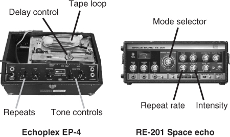
Figure 12.22 Tape Delay Signal Flow Architecture. The Space Echo provides up to three separate delays which are summed (as shown); the Echoplex features a single delay.
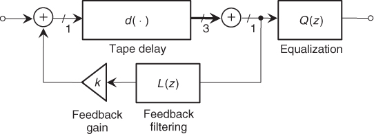
As seen in Figure 12.22, the input signal is delayed and fed back, with the delayed output equalized according to the tone controls. The amount of feedback is controlled by the “Repeats” knob, producing a loop gain k roughly in the range k ∈ [0, 2]. For loop gains less than one, the Echoplex produces a decaying series of echoes. With a loop gain greater than one, sound present in the system will increase in amplitude until saturating, and take on the bandpass spectral quality of the loop filtering, with a rhythmic temporal character determined by the delay setting. When k > 1, no input signal is needed to produce an output, as tape hiss and 60 Hz harmonics present in the system will cause the unit to self-oscillate.
The movable record head is capable of producing extreme Doppler shifts [AAS08]. If the delay control is quickly moved away from the playback head, the input may be Doppler shifted down sufficiently that the bias signal appears in the audio band. If the delay control is moved toward the playback head at a rate faster than the tape speed, a high-bandwidth transient will be recorded as the record head slows and is overtaken by the tape.
The Space Echo, released in 1973, is shown in Figure 12.21. It has similar controls to the Echoplex, but uses a variable tape speed controlled by its “Repeat Rate” knob to fix the time delay between the record and playback heads. As shown in Figure 12.23, the Space Echo has three playback heads whose outputs are summed according to the “Mode Selector” to form the delayed output.
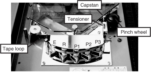
Figure 12.23 Space Echo Tape Transport. The erase (E), record (R), and three playback heads (P1, P2, P3) are shown.
Like the Echoplex, the Space Echo also has a saturating signal path, and a feedback loop gain k ranging from k ∈ [0, 2] according to “Intensity” control. Noise in the electronics will produce a self-oscillation similar to that of the Echoplex.
The Space Echo and Echoplex may be modeled according to their signal flow architecture, as shown in Figure 12.22. Unlike digital or electronic delays, the mechanics of the tape delay transport produce subtle fluctuations in the time delay which add to the character of the effect. In Section 12.5.2 below, the mechanics of the tape transport are described, and methods for simulating the time-delay trajectory are presented. In Section 12.5.3, details of the signal path are noted, including tape and electronic saturation, and an analysis of the tone control circuit.
12.5.2 Tape Transport
Delay Trajectories
The tape transport mechanism employed by the Space Echo and Echoplex uses a metal capstan engaged with a rubber pinch wheel to pull the tape past the record and playback heads. As seen in Figure 12.23, the tape is spliced into a loop, and passes through a tensioner before arriving at the pinch wheel and re-entering its cartridge. The various forces acting on the tape produce a tape speed which varies somewhat over time. This varying tape speed results in a fluctuating time delay, which adds to the character of the delayed signal and is important to the time evolution of the sound produced when the feedback gain is greater than 1.0. It should be pointed out that as the tape splice passes by the playback head, a modest dropout is produced.
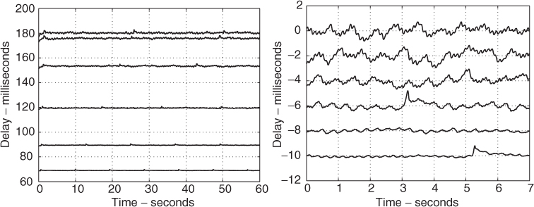
Figure 12.24 shows the time evolution of the time delays provided by the Space Echo playback head P1 measured at a variety of “Repeat Rate” (i.e., tape speed) settings. The resulting average time delays range from a little over 60 ms to a little over 160 ms. Figure 12.24 also shows the same delay trajectories with their means subtracted and offset for display. Both quasi-periodic and noise-like components are evident. Figure 12.25 shows spectra of the time-delay trajectories of Figure 12.24, plotted on frequency axes normalized according to their respective time delays. The spectra peak at the capstan rotation rate (about 22 Hz for the shortest time delay) and at the pinch-wheel rotation rate (near 3.5 Hz for the shortest time delay).
Figure 12.24 Space Echo delay trajectories (left), mean-subtracted trajectories, (offset, right).
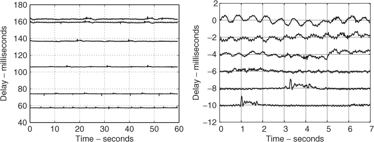
Figure 12.25 Delay trajectory spectra. Spectra of the delay trajectories of Figure 12.24 are plotted on frequency axes scaled to produce a 60 ms nominal delay.
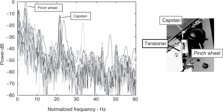
There are a series of nulls appearing near integer multiples of 15 Hz, and an overall low pass quality to the spectra. This pattern is reminiscent of a sinc function corresponding to a time-domain integration over a 60 ms window.
The 60 ms window length is precisely the (normalized) time delay, and represents the integration of velocity fluctuations as the tape travels between the record and playback heads. Tape speed disturbances completing an integer number of periods (slowing down and speeding up the tape) while traveling between the heads will have no effect on the resulting time delay, and therefore, do not appear in the time delay spectra.5
Another effect of the integration can be seen in Figure 12.24. Note that the longer the time delay, the longer the integration, and the greater the time-delay fluctuations. In fact, the amplitude of time-delay fluctuations is roughly proportional to the average delay.
In Figure 12.24, transients appear in the two time-delay trajectories offset at −10 ms and −8 ms. These temporary increases in time delay are the result of the tape splice squeezing through the tensioner and then the pinch wheel. The tape is temporarily slowed, and the time delay later temporarily increased. The passage of the splice—about once every nine seconds for the fast tape speed setting, and about every 27 seconds for the slow tape speed setting—is important for creating an evolving sound in the presence of heavy feedback.
Other factors influence the time-delay trajectory. Compared to the trajectories seen in Figure 12.24, measured using a new tape, the fluctuations when using old tape have a much larger stochastic component.
Delay Trajectory Physical Model
The delay trajectory may be generated using a model of the tape transport mechanics. The angular rotation rate of the capstan ωc is changed according to its moment of inertia I and applied torques,
In the above expression, τ(r) represents the motor torque applied as a function of the Space Echo “Repeat Rate” setting r (τ(r) is presumed constant for the Echoplex). The term μTρc is the torque resulting from the tensioner friction—it is the tape tension T, scaled by the coefficient of friction μ, acting at the capstan radius ρc. Rather than applying a constant torque according to μTρc, a unit-energy noise process is suggested, as this corresponds to the stochastic nature of frictional forces [Ser04].
The torque γ(θp) accounts for angular velocity changes due to the periodic deformation of the pinch wheel as it rotates about its axis. The distance between the capstan center and pinch-wheel axle is fixed, and any irregularities in pinch-wheel radius will result in corresponding deformations in the pinch-wheel rubber. Assuming a spring constant k, the energy stored in the pinch-wheel deformation at pinch-wheel angle θp is
12.40 ![]()
where ρp(θp) is the pinch-wheel radius at pinch-wheel rotation angle θp. In a time period Δt, the energy stored is
12.41 ![]()
The kinetic energy change ΔEω over the same time period is
12.42 ![]()
The pinch-wheel deformation results in a torque that balances the energy changes, ΔEs + ΔEω = 0,
12.43 ![]()
where the ratio of the capstan and pinch-wheel radii was substituted for the inverse ratio of their angular velocities. A source of pinch-wheel deformation is an off-center axle, generating a pinch-wheel radius
12.44 ![]()
where ρ0 is the pinch-wheel radius, and β is the distance of the pinch-wheel axle from the pinch-wheel center. This pinch-wheel radius generates the sensitivity
12.45 ![]()
The time delay δ(t) between the record and playback heads may be found by integrating the tape speed v(t) until the record head-playback head distance D is achieved,
12.46 ![]()
where v(t) is the tape speed produced by the spinning capstan. Compared to the global average tape speed v0, the tape speed fluctuations v(t)− v0 are small, and the varying time delay may be approximated by
where δ0 is the nominal delay, δ0 = v0/D. The time-delay trajectory is therefore the difference between the nominal delay and a running mean of the tape speed fluctuations.
Delay trajectories synthesized using (12.39) and (12.47) are shown in Figure 12.26, along with the corresponding delay fluctuations. A simple tape splice model was included.
Figure 12.26 Space Echo synthesized delay trajectories (left), mean-subtracted (offset, right).
Delay-trajectory Signal Model
The fluctuating time delay driving the tape-delay model may be formed without reference to the mechanics of the tape transport. Instead, the observed time-delay trajectory characteristics may be reproduced via a “signal model.”
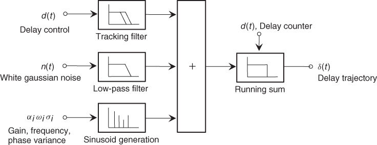
In this approach, the tape delay is formed, as shown in Figure 12.27, by adding the three time-delay trajectory components: a mean delay, as determined by the delay control position for the Echoplex or the “Repeat Rate” for the Space Echo; quasi-periodic processes representing the observed capstan and pinch-wheel harmonics; and a stochastic low-frequency drift. This sum is filtered via a running mean having length equal to the time delay. The pinch-wheel and capstan components are generated by summing sinusoids at integer multiples of the observed capstan and pinch-wheel rotation rates, with amplitudes equal to those seen in the measured time-delay fluctuation spectra. The sinusoid phases are incremented according to their respective measured frequencies, with small low pass, zero-mean noise processes added to the sinusoid phases to introduce observed frequency fluctuations. The low-frequency drift component is formed by filtering white Gaussian noise.
Figure 12.27 Delay trajectory signal model.
Delay Control Ballistics
As described above, the Space Echo time delay is controlled by adjusting the speed of the motor driving the capstan-pinch wheel assembly; the Echoplex time delay is controlled directly by positioning the record head. In both of these controls, there is a time lag between when the control is moved and when the desired delay is reached. This is seen in Figure 12.28 for the case of the Space Echo having its “Repeat Rate” control quickly adjusted between its slowest and fastest settings.
Figure 12.28 Space Echo delay trajectory, stepped “Repeats Rate” control.
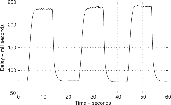
The behavior seen in Figure 12.28 is well approximated by a so-called leaky integrator: a target signal vT is tracked to produce v(n) using a first-order update,
12.48 ![]()
where λ, the “forgetting factor,” governs the rate at which the target signal vT replaces the current estimate v(n). With λ near 0, the target vT quickly replaces the integrator output v(n), whereas with λ near 1, the integrator output slowly relaxes to the target. Given a time constant τ and sampling rate fs, the forgetting factor
12.49 ![]()
will produce a leaky integrator, whose output will be a factor 1− 1/e closer to a constant target signal after a period of time τ.
Referring again to Figure 12.28, the tape speed is seen to relax to its target value with a time constant on the order of 1 second when the target tape speed is greater than the current tape speed. However, when the target tape speed is less than the current tape speed, the time constant is slower at about 2 seconds. This behavior may be captured using different forgetting factors, depending on whether the target tape speed is greater than or less than the current tape speed.
Time-varying Delay Implementation
For arbitrary interpolated delay-line access, it is convenient to use Lagrange interpolation, since the needed filter coefficients can be calculated inexpensively for any fractional delay [Laa96]. The Lagrange interpolation filter is defined as the FIR filter which models the ideal fractional delay e−jδω with a maximally flat approximation at DC. In other words, for a fractional delay of δ, the Nth-order Lagrange filter will have a frequency response H(ejω) which matches e−jδω and its first N derivatives at ω = 0. Usually, the M-tap Lagrange filter will be used to produce a delay δ such that M/2 < δ < M/2 + 1 for even M.
The ideal fractional delay e−jδω has nth derivative (− j)nδn at ω = 0. The Nth-order FIR filter has a frequency response
12.50 
which has nth derivative
12.51 ![]()
at ω = 0. Matching the response and first N derivatives of H(ejω) at DC to those of the ideal fractional delay defines the filter coefficients bn for the desired delay δ,
12.52 ![]()
where V is the Vandermonde matrix defined by the row [0 1 2 ⋯ N], ![]() is the column of filter coefficients [b0 b1 b2 ⋯ bN]T, and
is the column of filter coefficients [b0 b1 b2 ⋯ bN]T, and ![]() . For N = 3, we have
. For N = 3, we have
12.53 
The filter coefficients ![]() can be found by inverting V,
can be found by inverting V,
12.54 ![]()
For real-time operation, the matrix inversion can be carried out in advance. The product ![]() allows efficient calculation of bn for a given fractional delay δ. As the filter order N increases, the Lagrange interpolator coefficients converge towards a sampled sinc function, which would give ideal bandlimited interpolation.
allows efficient calculation of bn for a given fractional delay δ. As the filter order N increases, the Lagrange interpolator coefficients converge towards a sampled sinc function, which would give ideal bandlimited interpolation.
M-file 12.9 (lagr2.m)
% lagr2.m
% Authors: Välimäki, Bilbao, Smith, Abel, Pakarinen, Berners
% lagr.m -- Lagrange filter design script
fs=44100;
numtaps=8; %% Make this even, please.
ordvec=[0:numtaps-1]';
VA=flipud(vander(ordvec)'),
iVA=inv(VA); %matrix to compute coefs
numplots=16;
for ind=1:numplots
eta=(ind-1)/(numplots-1); %% fractional delay
delay=eta+numtaps/2-1; %% keep fract. delay between two center taps
deltavec=(delay*ones(numtaps,1)).∧ordvec;
b=iVA*deltavec;
[H,w]=freqz(b,1,2000);
figure(1)
subplot(2,1,1)
plot(w*fs/(2*pi),(abs(H)))
grid on
hold on
xlabel('Freq, Hz')
ylabel('magnitude')
axis([0 fs/2 0 1.1])
subplot(2,1,2)
plot(w*fs/(2*pi),180/pi*unwrap(angle(H)))
grid on
hold on
xlabel('Freq, Hz')
ylabel('phase')
xlim([0 fs/2])
end
figure(1)
subplot(2,1,1);hold off;
title('Lagrange Interpolator')
subplot(2,1,2);hold off;
12.5.3 Signal Path
Recording with AC Bias
Magnetic data storage is achieved by exposing magnetic material to an external magnetic field. If the applied field is of sufficient magnitude, residual magnetization of the material will persist after the external field is removed. For a time-varying field applied along a single axis to a magnetic material, the relationship between the applied field and the magnetization of the material will take the hysteretic form shown in Figure 12.29. A demagnetized sample will follow trajectory ‘1’ in the figure if an increasing magnetic field is applied. The magnetization will grow to a maximum Ms for large fields, where Ms is the saturation magnetization for the material. As the applied field is reduced, the magnetization will decrease along trajectory ‘2’ until, at an applied field of zero, the magnetization will be Mr, the remanent magnetization for the material. When the applied field reaches the coercive force −Hc, the total magnetization of the sample will once again be zero. If the applied field becomes more negative, the sample will continue to follow trajectory ‘2’. If, at a later time, the applied field is once again increased, the sample will follow trajectory ‘3’.
Figure 12.29 Hysteretic magnetization curve, showing saturation magnetization Ms, remanent magnetization Mr, and coercive force Hc.
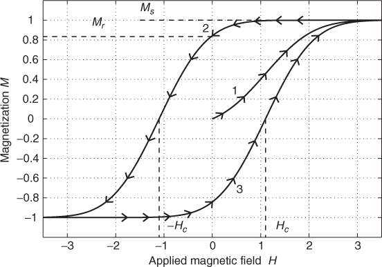
The hysteretic process of Figure 12.29 leads to a highly nonlinear relationship between the applied field and the resultant magnetization. In order to linearize the recording process, an AC bias signal consisting of a high-frequency sinusoid is typically added to the audio signal. The sum of the two signals is passed to a record head which creates a localized magnetic field that is proportional to the current passing through it.
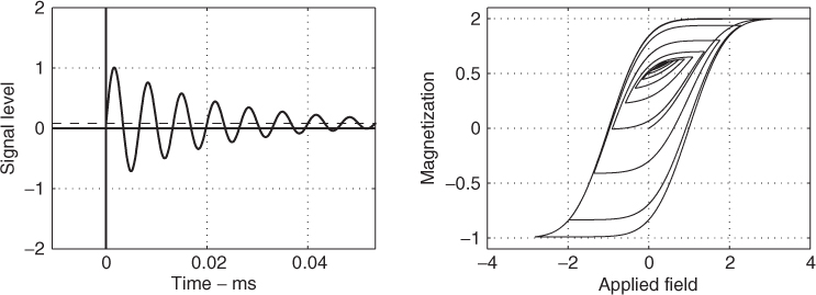
When an element of tape moves past the record head, it is exposed to the magnetic field created by the head. As the tape recedes from the head gap, the field applied to the tape becomes progressively weaker through distance, and the tape element experiences a decaying, oscillating magnetic field due to the AC bias. If the audio signal is bandlimited to frequencies much lower than the AC bias frequency, it can be considered quasistatic during the decay of the bias field. For a decaying AC bias signal added to a quasi-DC signal, the field applied to the tape would be as shown on the left of Figure 12.30. This signal produces the magnetization trajectory shown on the right-hand side of the figure. The trajectory spirals inward to a final magnetization which is largely insensitive to the details of the bias signal, and depends only upon the value of the quasi-DC component. In this way, the hysteretic behavior is eliminated, resulting in what is known as the anhysteretic recording process.
Figure 12.30 Anhysteretic recording. Decaying AC bias signal plus DC offset (left). Magnetization trajectory for decaying signal (right).
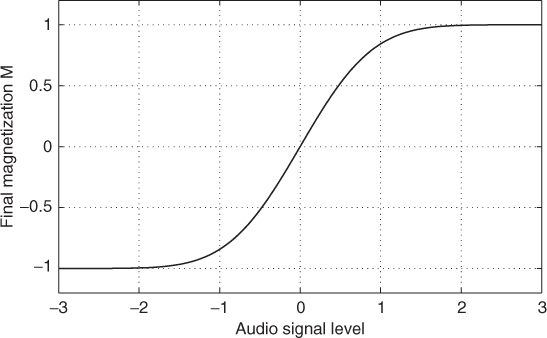
In reality, the audio component of the record signal will decay along with the bias signal as the tape element moves out of the recording head gap, producing the signal and magnetization trajectory of Figure 12.31. This is known as the modified anhysteretic recording process [Mal87]. With the hysteresis eliminated, the record process can be modeled as a memoryless nonlinearity. With proper biasing levels, recordings can be made with very little distortion, as long as levels are kept below Ms. The anhysteretic recording nonlinearity can be approximated by the error function M = erf(H), shown in Figure 12.32.
Figure 12.31 Modified anhysteretic recording. Decaying AC bias signal and signal (left). Magnetization trajectory for decaying signal (right).
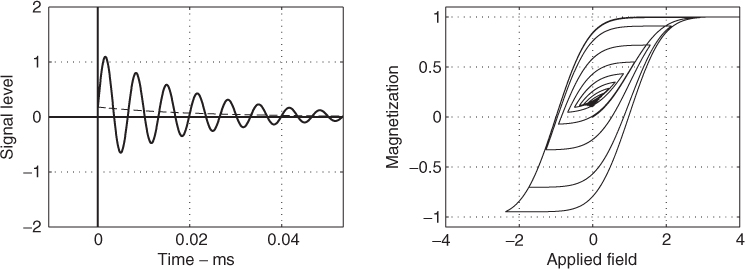
Figure 12.32 Memoryless nonlinearity for anhysteretic recording.
Tape-speed-dependent Equalization
For signal reproduction, the tape is dragged across a gapped play-head which detects changes in magnetization as the tape goes by. The head is most sensitive to the space immediately surrounding the gap, but also responds to more distant elements of the tape. The recovered signal can be calculated as the derivative in time of a weighted volume integral over the space surrounding the head. The sensitivity of the head depends upon field direction as well as spatial position. This is reflected by taking a dot product between the tape magnetization and a vector representing the head's (directional) sensitivity as a function of space. The recovered signal s can be expressed as
12.55 ![]()
where ![]() represents the head's sensitivity.
represents the head's sensitivity.
The spatial integration performed by the playback head leads to wavelength-dependent equalization. At high frequencies, the wavelength recorded on tape becomes comparable to the gap width in the head, leading to a sinc-like frequency response; when an integral number of wavelengths fits in the gap, the response is diminished. This effect is called gap loss and takes the form
12.56 ![]()
where γ(k) is the wavelength-dependent gain, k is the wavenumber, and g is the width of the head gap. A related effect happens at low frequencies when the wavelength becomes comparable to the dimension of the head core. This is called the contour effect, and produces what is known as head bump. Both gap loss and the contour effect are influenced by tape speed v, since k∝1/v. For the Roland Space Echo, since delay times are adjusted by changing the tape speed, the equalization will depend on delay. For the Echoplex, the tape speed is relatively constant, and the equalization will not be affected by delay setting.
Electronics
Equalization is applied electronically before writing to tape, and again after reading back from tape. This is done to maximize the tape's dynamic range, and to minimize the spectral coloration associated with the record/playback process. The equalization at the record head can be measured directly if the AC bias source is temporarily disconnected. The record head itself presents an inductive load over most of the audio band. At low frequencies, the series resistance of the head windings can become dominant. The field applied to tape is proportional to the current through the head, which can be measured directly or calculated from the head voltage if the head impedance is known. In many cases the high-frequency content of the signal is emphasized at the record head. It should be noted that at some frequencies the amplifier circuit will clip before reaching the level required to saturate the tape. This can be observed with both the Space Echo and the Echoplex.
After playback, the signal is equalized to give the desired transfer function, as measured from input to output. For the Space Echo and Echoplex, the overall equalization is relatively flat, and bandlimited. Plots of the equalization as a function of tape speed for the Space Echo are shown in Figure 12.33.
Figure 12.33 Space Echo equalization, various tape speeds (left), Echoplex loop equalization (right).
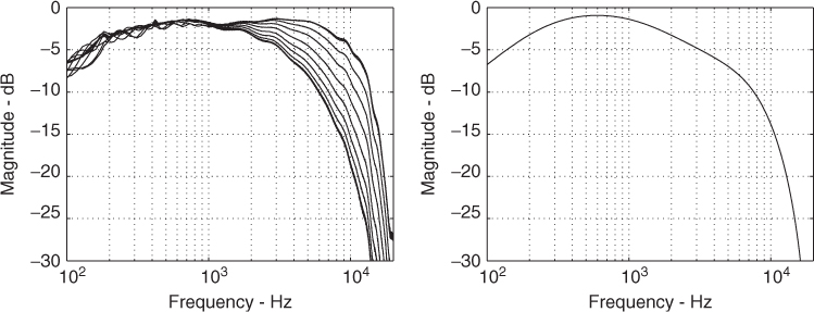
When in feedback mode, the Space Echo and Echoplex have an overall equalization associated with one trip around the feedback loop. This equalization can be measured by taking spectral ratios between successive echoes of a broadband signal. The loop equalization is the concatenation of parts of the pre-record and post-playback equalization, along with whatever equalization is present in the feedback path. The loop equalization for the Echoplex is plotted in Figure 12.33.
Tone Controls
Tone controls are present on both the Space Echo and Echoplex, and affect the output equalization. Neither unit places the tone controls within the feedback loop. The Echoplex tone circuit is as shown in Figure 12.34. In the figure, ‘B’ refers to the position of the bass tone control, where B = 1 for full boost and B = 0 for full cut. The marking ‘T’ indicates the position of the treble control. Measured frequency responses for various control settings are plotted in the same figure.
Figure 12.34 Echoplex EP-4 tone circuit and frequency response.
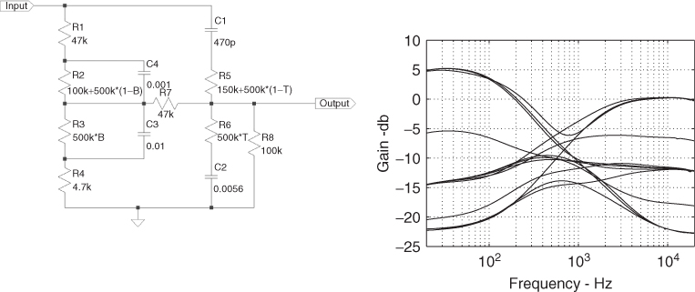
This circuit is related to the Baxandall tone circuit [Bax52] and provides high and low shelving functions. The Baxandall circuit is common in hi-fi and guitar tone stacks. Because of the topology of the circuit, the transfer function cannot be directly computed using series-parallel combinations of the components. However, superposition can be used to decompose the transfer function into two components, each of which can be calculated in a straightforward way. The two superposition components are shown in Figure 12.35.
Figure 12.35 Echoplex EP-4 tone circuit superposition components.
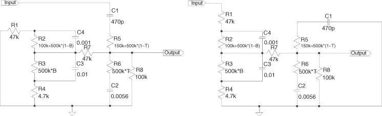
The circuit transfer function is identically equal to the sum of the transfer functions of the two superposition components. Because of the topologies of the components, the two transfer functions have the same poles, so that the numerator terms can be added directly. As can be seen, each of the two components can be evaluated directly using series-parallel combinations.
Alternatively, the circuit can be analyzed using the n-extra element theorem (nEET) [Vor02]. Using nEET, the terms of the numerator and denominator of the transfer function can be calculated directly by inspection, using driving-point impedances associated with the reactive components of the circuit.