Electro-magnetics and mathematical model of magnetic bearings
In this chapter, basic structures, analyses and mathematical models of magnetic bearings and related actuators are presented in addition to the following. The principles of a feedback control strategy for magnetic bearings are introduced, and a simple electromagnetic actuator is developed in order to understand the electrical equivalent circuits. An analysis is carried out that calculates the inductance, flux densities, stored magnetic energy and magnetic forces. Typical structures for the radial magnetic bearing and related actuators are described. As a result of the analysis, a simple representation of the magnetic bearing is introduced. The maximum radial force is also derived based upon the saturated flux density in the magnetic circuits. A block diagram is drawn in order to develop a controller.
2.1 Electro-mechanical structure and operating principles
Figure 2.1 shows the basic structure of an electromagnet with a feedback controller for one-axis magnetic suspension. Excitation of the winding produces a magnetic force to suspend the rectangular iron object. The object is free only in the vertical axis. The current i produces a flux ψ. The flux path is shown by the dotted line and it crosses the airgap twice in the vertical direction. The attractive force between the suspended object and C-core is a function of i, and is proportional to the square of i if the core is not saturated. Under steady-state conditions, the generated attractive force is adjusted to be exactly equal to the product of the object weight m and gravity acceleration ga to satisfy the force equilibrium.
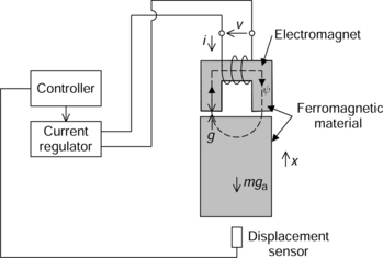
The displacement sensor detects the vertical position of the suspended object. The sensor output voltage is the input to a controller. A magnetic force command is generated to stably suspend the object. The force command is the sum of damping- and spring-force commands. The damping-force command is proportional to the speed of the suspended object. The spring-force command is proportional to the displacement of the suspended object. These commands are in the opposite direction to the speed and displacement for negative feedback. The controller generates a current command so that the generated force follows the force command. The current regulator controls the current by applying a voltage to the electrical terminals.
The current i excites a series-wound coil. Let us suppose that the number of turns in the winding is N so that a magneto motive force (MMF) Ni is produced. Since the permeability is high in ferromagnetic materials, the flux follows the path shown. The flux crosses the airgap twice. Note that only one flux path is shown; however, the flux is distributed in the airgap. The maximum flux density in the airgap determines the force capability of the electromagnet. A high flux density results in high magnetic force. However, the maximum flux density is limited to 1.7 to 2 T in conventional silicon steel. It is also important to make the airgap length as small as possible, which will reduce the current and losses.
2.2 Electric equivalent circuit and inductance
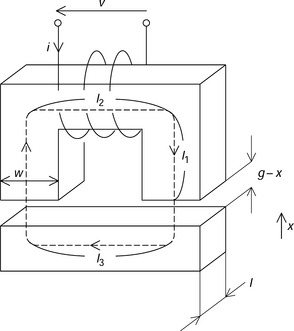
Figure 2.2 shows an electromagnet used to suspend an I-shaped core with a magnetic force. The C-core has a width w with a stack length l. The main flux path is indicated by the dotted line. The lengths of the flux path in the C-core are defined by l1 and l2. The flux path length in the I-shaped core is l3. The winding has N turns. The instantaneous current value is i, so that the MMF is Ni. The airgap length is g at the nominal position. A coordinate position x is defined in the I-shaped core position so that the airgap length is (g − x). The reluctance of the magnetic circuit is defined as
where:
A permeance is the inverse function of magnetic reluctance, i.e., for a permeance
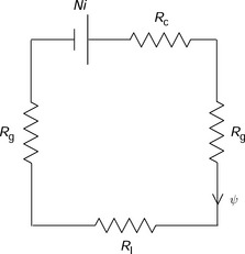
Figure 2.3 shows an “electrical” equivalent circuit for the magnetic circuit of the electromagnet. In terms of MMF (voltage), flux (current) and reluctance (resistance), a constant (dc) magnetic circuit can be treated in the same way as an electric circuit. The main difference is that magnetic reluctance is an energy storage component rather than a loss component. The “dc voltage” source Ni represents the MMF generated by the winding current. Rc and RI are the magnetic reluctances in the C- and I-cores, respectively, and Rg represents the magnetic reluctance at the airgap. These magnetic reluctances are written as
where μ0 is the permeability of free space (μ0 = 4π × 10−7 H/m) and μr is the relative permeability (μmt = μr.μ0). The value of μr. for iron is typically in the range of 1000–10000. The relative permeability of air is approximately equal to 1.0. In most cases, the airgap reluctance is significantly larger than the iron reluctance, so that the magnetic reluctance in the iron can be neglected in the following calculation. Therefore the equivalent electrical circuit is simplified. The flux ψ is then
The flux linkage λ1 of the coil is defined as the number of turns N multiplied by the flux passing through the coil:
But inductance is defined as flux linkage divided by the current value (L =λ1/i), giving
If the displacement x is small compared to the airgap length, the following series expansion is applicable
and if only the first and the second terms are considered, the inductance can be approximated to
where L0 is defined as the nominal inductance
In addition, the flux density B in the airgap can be derived as
Calculate the magnetic reluctances when x = 0, assuming the following dimensions: w = 1cm, l = 1cm, l1 = 1cm, l2 = 3 cm, l3 = 4 cm and g = 1 mm. Assume the relative magnetic permeability in the iron μr = 1000.
From the dimensions given above, the magnetic reluctances can be calculated: Rg = 8 × 10⁶ A/Wb, Rc = 5.6 × 10⁵A/Wb, RI = 3.1 × 10⁵A/Wb. The airgap reluctance is dominant since Rg ![]() Rc + RI.
Rc + RI.
2.3 Stored magnetic energy and force
In this section, the magnetic force is derived at an arbitrary displacement by consideration of the stored magnetic energy in the system. The concept of co-energy is also introduced and several simple examples of actuators are shown.
Figure 2.4 shows a relationship between the flux linkage λ and current i in magnetic circuits with ferromagnetic components such as the cores in Figure 2.2.
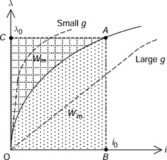
The flux linkage is proportional to the current only at low current values. At high current, the ferromagnetic cores become saturated, producing a nonlinear characteristic. In conventional silicon steel, magnetic saturation occurs at a flux density between 1.2 and 1.8 T. The exact saturation curve depends on the type of silicon steel. Such information is provided by the steel manufacturer.
The magnetization curves also depend on the airgap length between the C- and I-cores. With a small airgap length, the λ/i curve is quite nonlinear because the magnetic circuit is dominated by the saturable C- and I-core reluctances at high current. A wide airgap length results in a more linear characteristic because the circuit reluctance is now dominated by the airgap reluctance component even at high current, which is non-saturable.
Let us suppose that the operating point is A in Figure 2.4, with current i0 and flux linkage λ0. The stored magnetic energy Wm in a magnetic system is obtained from

The integration corresponds to the area bounded by points O, C and A. In addition to the magnetic energy, we can introduce the magnetic co-energy W′m. The magnetic co-energy is defined as

This definition indicates that the magnetic co-energy is represented by the area bounded by points O, B and A. The sum of Wm and W′m is equal to a product of current i0 and flux linkage λ0. Wm is the stored magnetic energy in the system whereas the co-energy is a component we introduce to aid analysis but has no physical reality.
The independent variables in a magnetic suspension system are normally the winding current and object displacement. If the system is moved by δx then it can be shown that the work done is equal to the change in co-energy of the system. Since the work done is the force F × δx, the electromagnetic force F is given as the partial derivative of the magnetic co-energy
This equation provides the expression for the electromagnetic force between the C- and I-cores with nonlinear magnetizing characteristics.
If the magnetizing characteristic curve is linear (i.e., no saturation) then the flux linkage and current relationships are as shown in Figure 2.5. It is seen that magnetic energy and magnetic co-energy are equal so that
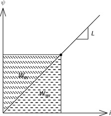
In this instance, the magnetic force can be also written as
Note that this equation is valid only for a magnetically linear system.
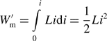
Assuming a linear system, where the self-inductance L is constant and Li = λ, the magnetic co-energy W′m is derived as
The electromagnetic force F is
From (2.10), the partial derivative of L with respect to x is
Substituting (2.20) into (2.19) yields
2.3.1 Flux density and electromagnetic force
In equation (2.21), the magnetic force is expressed as a function of current. Another useful expression obtains the force from the flux density in the airgap. L0 in equation (2.21) is substituted by (2.11) so that
Assuming that x = 0, solving (2.12) for Ni yields
Therefore substituting (2.23) into (2.22) produces
But 2wl is the area of airgap. Let us define the airgap area S as 2wl so that the magnetic force is expressed as in the well-known Maxwell stress equation where
This equation gives us a straightforward insight into magnetic force generation. It can be said that the magnetic force is proportional to the square of flux density in the airgap. The force is also proportional to the airgap area. The following example provides a practical way to estimate the magnetic force.
Consider the arrangement in Figure 2.6 and answer the following questions:
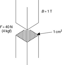
1. At flux density of 1 T, derive the magnetic force assuming S = 1cm2.
2. At the same flux density, derive the magnetic force at S = 1m2.
3. Suppose that the saturated flux density in silicon steels is 1.7 T. How much radial force is generated for S = 1cm2?
1. F = 12/(2 × 4π × 10−7) × 100 × 10−6 = 40N(≅ 4 kgf). Remember that the flux density level in the airgap is usually less than 1 T so that a magnetic force density of 40 N/cm2 (approximately 4kgf/cm2) gives the highest practical value. Figure 2.6 illustrates this. There is an airgap between two iron poles. The flux density is 1 T and the area under the poles is 1 cm2 so that there is an attractive force of 40 N between these two poles.
3. 116N (≅ 12kgf). If the flux density in the airgap is increased to 1.7T then the magnetic force is three times the value at 1 T. To achieve 1.7 T, an extremely high MMF is usually required. Increasing the MMF may possibly require bulky coil windings and external cooling. Engineers usually find that it is more practical to increase the airgap area rather than flux density.
2.3.2 Nonlinear magnetic characteristics
So far we have considered the magnetic force by assuming that iron cores have linear characteristics, i.e., the permeability is constant. It is also assumed that the iron permeability is high so that the iron core reluctance can be neglected. However, in some cases, the core reluctance should be considered. For example, a magnetic circuit with a very short airgap length but long flux path in the iron core has high per-unit iron reluctance. In this case, the relationship between flux linkage and current is highly nonlinear.
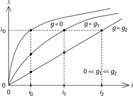
Figure 2.7 shows magnetization characteristics of a C- and I-core combination under three different conditions. Without an airgap, the magnetization curve is determined by the nonlinear magnetic characteristics of the iron core. If a small airgap is introduced, the flux linkage is decreased for a given current because the airgap results in an increase in magnetic reluctance. If the airgap is further increased, the magnetization curve becomes straight because the magnetic reluctance is mainly due to the airgap reluctance. In this case, we can assume a linear characteristic; however, it has to be noted that more current is required to achieve the same flux linkage level. For example, to achieve λ0, the currents i0, i1 and i2 are needed for g = 0, g1 and g2, respectively. In order to reduce copper losses and coil dimensions, the airgap length is usually made as small as possible.
2.3.3 Force calculation in nonlinear magnetization curve
We have derived two force equations. One is based on the current and the other is based on the flux density in the airgap. These are (2.21) and (2.25), and are repeated here:

Let us see how accurate these equations are under magnetically saturated conditions.
Figure 2.8(a) shows nonlinear magnetization curves of a C- and I-core with a small airgap using a piece-wise linear approximation. At low current, the relationship between the flux linkage and current is linear. The derivative of flux linkage with respect to the current is the self-inductance L. At high current, the core is saturated. Suppose the operating point is A with 0, and i0 at the airgap length of xA. Let us suppose that the airgap length is increased by Δx so that the magnetization curve is moved to line OB for xA + Δx. The area OAB bounded by the magnetizing curves at x = xA and xA + Δx is the co-energy variation ΔW′m. A product of the magnetic force and the displacement Δx is equal to the area ΔWΔm. Hence the shaded area is proportional to the magnetic force.
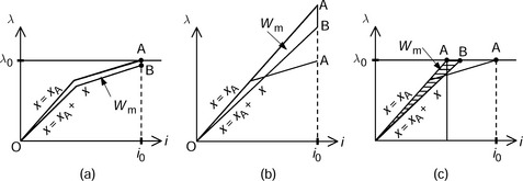
Figure 2.8 Linear approximation errors: (a) nonlinear system co-energy; (b) magnetic co-energy in a magnetically linear model based on current value; (c) magnetic co-energy in a magnetically linear model based on flux linkage value
In Figure 2.8(b) the co-energy obtained from the current equation is shown. The equation assumes a linear relationship even at high current. At the current i0, the flux linkage is Li0 so the operating point is A′. The shaded area OA′B′ is the co-energy ΔW′m. We can see that the calculated ΔW′m is too high. Therefore the magnetic force calculated from (2.21) is higher than the actual values under saturated conditions.
In Figure 2.8(c) the co-energy based on the flux density equation is shown. Again, the magnetization curve is the extension of linear relationship, i.e., λ = Li. Since the flux density is proportional to the flux linkage, even in the nonlinear conditions, the operating point is A″ with flux linkage of λ0. Therefore the shaded area OA″B″ is the co-energy variation. One can see that ΔW′m is smaller than that in Figure 2.8(b). Hence the overestimation of magnetic force can be avoided under saturated conditions. Equation (2.25) is widely used in estimating the achievable magnetic force to avoid overestimation.
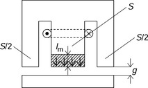
2.3.4 Differential actuator
Figure 2.9 shows a differential type of magnetic actuator. The cylindrical object can move in the x direction. It is suspended in the air by a controlled magnetic force. Two C-shaped actuators are used as illustrated. Suppose that the flux distribution in the airgap is uniform with flux densities of B+ and B− in the upper and lower airgaps respectively. The airgap area is S with a sum of S1 and S2. The magnetic forces F1 and F2 are applied to the cylindrical object. These forces are F1 = B2+S/(2μ0) and F2 = B2−S/(2μ0) so the sum of these magnetic forces F is written as
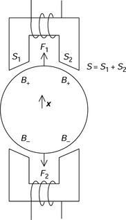
It can be seen that the magnetic force is proportional to the difference of flux density squared.
Suppose that B+ = B0 + ΔB and B− = B0 − ΔB, i.e., these flux densities are controlled by the bias flux density B0 and differential flux density ΔB. The object weight is supported by a magnetic force. Derive B+,B−, ΔB, F1 and F2 assuming that S = 2cm2, B0 = 0.5T and the weight of the cylindrical object is 1 kg.
Substituting B+ = B0 + ΔB and B− = B0 − ΔB into (2.26), one can derive
Substituting F = 9.8N and the given values we get ΔB = 0.062 T. Hence B+ = 0.562 T, B− = 0.438 T, F1 = 25.14N and F2 = 15.27N.
2.3.5 Surface-mounted permanent magnet motor (SPM motor)
Figure 2.10 shows a permanent magnet motor. On the rotor, a cylindrical-ring permanent magnet is mounted on the shaft. The permanent magnet is pre-magnetized with two poles. On the stator, there are four salient poles. Each pole has a winding; however, only one phase winding is shown in the Figure 2.10. Motor fluxes are produced by the permanent magnets. Therefore attractive magnetic forces exist between the rotor surface and stator poles. Normally, the sum of these forces is zero if the rotor is centred, and the currents in opposite coils are equal or zero.
A machine has a rotor with a diameter of 50 mm with an axial length of 50 mm. Let us suppose that the flux density distribution in the airgap between the rotor and stator poles is uniform with a peak of 0.7 T. The rotor is made of NdFeB permanent magnet and silicon steel. The mass density of these materials can be averaged to 7.65 g/cm3.
1. Find airgap area of one stator pole.
2. Find magnetic force between one stator pole and the rotor.
3. What is the ratio of magnetic force to the rotor weight?
4. Find total magnetic force acting on the rotor.
5. Suppose that the flux density in the airgap of stator poles 1 and 3 are actively controlled as in the example shown in Figure 2.9. Find the ΔB necessary to support a rotor.
2. The magnetic force is F = 4kgf/cm2 × (0.7T)2 × 13.1cm2 = 25.7kgf.
3. The rotor volume is ![]() . The density of silicon steel and permanent magnet is approximated to 7.65g/cm3, therefore the weight is 0.750 kg. This means that the magnetic force at one stator pole is about 34 times the force exerted by the rotor weight.
. The density of silicon steel and permanent magnet is approximated to 7.65g/cm3, therefore the weight is 0.750 kg. This means that the magnetic force at one stator pole is about 34 times the force exerted by the rotor weight.
4. Total magnetic force acting on the rotor is zero because radial forces under stator poles 1 and 3 cancel each other out. The forces under poles 2 and 4 also cancel.
5. Substituting F = 0.750 × 9.8N, S = 13.1 × 10⁻⁴ cm2 and B0 = 0.7T into ![]() gives ΔB = 0.005 T.
gives ΔB = 0.005 T.
In this example, we can see that significant attractive forces are generated between the rotor and the stator salient poles. There are disadvantages and advantages with these radial forces as described below.
If an electrical motor shaft is misaligned from the rotor centre position so that it no longer rotates on its own axis, the four radial forces are unbalanced so that total magnetic force is no longer zero. The generated magnetic force rotates with the rotor. This rotating radial force results in vibrations and acoustic noise and it also shortens the bearing life.
If the radial magnetic forces in the four stator poles are actively controlled then a rotor shaft can be supported by magnetic forces. A slight unbalance of flux density of 0.005 T generates a magnetic force which will suspend the rotor weight. Even if the rotor experiences a centripetal force of 9 G, a flux density variation of only 0.05 T is sufficient to suspend the rotor.
2.3.6 E- and I-cores with a permanent magnet
Figure 2.11 shows E- and I-shaped iron cores with a permanent magnet. The permanent magnet is characterized by the residual flux density Br, which is in the range 1–1.45 T for rare-earth permanent magnets employing Neodymium or Samarium, and about 0.5T (or less) for low-cost ferrite permanent magnets. The flux generates an attractive force between the E- and I-cores. The permeability (called the recoil permeability μrec) of a permanent magnet depends on the magnet’s material but is generally slightly greater than one for rare-earth magnets.
Derive the magnetic force using the following procedures and answer the following questions:
1. Assume a one-turn coil in the E-core as shown. Obtain the coil current which generates the same flux as the permanent magnet. Assume that the residual flux density of the magnet is Br, the magnet thickness is lm, the flux path area is S and the airgap length is g. Also assume that the iron reluctance and leakage and fringing fluxes are negligible and that the magnet recoil permeability is one.
2. Derive the self-inductance of the one turn coil.
4. Find the flux density in the airgap.
5. How can we increase the magnetic force?
6. Suppose that both a permanent magnet and a winding are used in this electromagnet. A static force is provided by the permanent magnet MMF and, in addition, a dynamic force is provided by the winding current MMF. Find the electromagnetic force. If the permanent magnet is very thin, the force/current is low because of low flux density in the airgap. If the permanent magnet is thick, the force/current is low because of the high magnetic reluctance of the permanent magnet. Find the condition for maximum force/current.
Apply the numerical parameters of S = 1cm2, Br = 1T, lm = 1 mm and g = 0.5 mm.
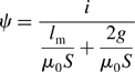
1. Figure 2.12 shows a magnetic equivalent circuit of the E- and I-cores. The airgap reluctances are g/(μ0S) and 2g/(μ0S) while lm/(μ0S) is the permanent magnet reluctance. The permeability of the permanent magnets is not exactly equal to that of free space, e.g., μr. = 1.05 for NeFeB; however, it can be approximated to unity. The current of the supply is also the MMF of the one-turn coil with current i.
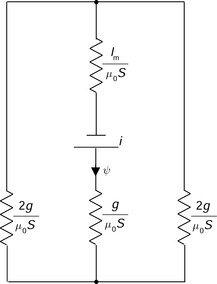
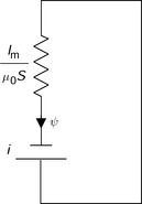
Let us suppose that the airgap length is zero. The equivalent circuit is then simplified as shown in Figure 2.13. The permanent magnet is short-circuited and the flux ψ is obtained from ψ = μ0Si/lm Hence the flux density B in the permanent magnet is given as B = ψ/S = μ0i/lm. This flux density is equal to the residual flux density Br so that
Substituting with the given numerical parameters gives i = 800 A.
2. In Figure 2.12, the flux is written as
The self-inductance is derived from the flux per unit current so that
3. From the inductance L and current i, the magnetic energy is equal to Li2/2. Substituting this into (2.29) yields
Assuming a magnetically linear flux path, the magnetic force F is the partial derivative of the energy with respect to the airgap length F = δWm/δg. Thus
Note that the direction convention of the magnetic force is opposite to the coordinate of displacement g so we change the polarity. The current i is substituted from (2.27), giving
Using the given parameters, F = 19.9N.
4. The flux density is obtained from the flux in (2.28) divided by the area S, and substituting into (2.27) gives B = [lm/(lm + 2g)] × Br. The flux density is 0.5 T.
5. One way to increase the magnetic force is to increase the permanent magnet thickness. An increase in lm results in an increase in the airgap flux density. In the flux density equation, the coefficient is 0.5; however, this value can be increased to nearly 1.0 by an increase in lm. It can also be noticed that a decrease in the airgap length also increases the airgap flux density. Another way to increase the magnetic force is to use a stronger permanent magnet with high residual flux density. In this example, Br = 1 T; however, magnets with Br up to 1.45 T are available on the market.
6. Let us define the current in the one-turn coil as ic. Let us also define the equivalent current caused by the permanent magnet as Ip. Then, the coil current is a sum of the actual coil current and the equivalent permanent magnet current so that i = Ip + ic = Brlm/μ0 + ic (from 2.27). Substituting this current into (2.31):
This equation shows that the force is not a linear function of coil current. In most cases, linearization is carried out near the operating point so that the maximum radial force for the current ic can be obtained from a partial derivative of F with respect to ic. The partial derivative of F can be derived as
The optimum permanent magnet thickness which maximizes the force/current is given when the partial derivative of the above equation is zero.
The above equation gives several solutions for permanent magnet thickness lm; however, only one reasonable solution is obtained. Assuming that coil current is much smaller than the equivalent permanent magnet current, the equation simplifies to
The result of this equation indicates that the maximum radial force for a given winding current is obtained if the permanent magnet thickness is twice the airgap length. This fact gives us a simple criterion when designing a permanent magnet-assisted magnetic suspension system such as a zero power magnetic suspension system.
7. Let us define x as a displacement from the reference airgap between the E- and I-cores. The airgap length is expressed as g − x. With no coil current the magnetic force is dependent on x so that (2.31) can be re-written as
The force and displacement have a nonlinear relationship. Thus, the partial derivative of the force with respect to x gives force/displacement around the operating point. Solving the derivative and substituting Ip into i in (2.27) yields
the condition at x = 0 can be obtained, where
Hence the force/displacement is maximum when the permanent magnet thickness is four times the nominal airgap length. In some cases, increasing the force/displacement is important because of the wide frequency response requirement for the magnetic suspension system.
2.4 Radial magnetic bearing
In this section, the principles, basic analyses, examples and linearization of a typical 8-pole radial magnetic bearing are described and discussed.
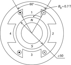
Figure 2.14 shows the cross section of a typical radial magnetic bearing. The rotor is cylindrical in shape with a centre shaft surrounded by ferromagnetic material such as laminated silicon steel. The stator surrounds the rotor and has eight poles. The areas between the stator poles are the slots and contain the windings. The stator yoke completes the magnetic paths of the eight stator poles. The width of the stator yoke is designed to be wide enough to avoid magnetic saturation and produce high mechanical stiffness in order to avoid vibration caused by radial magnetic forces.
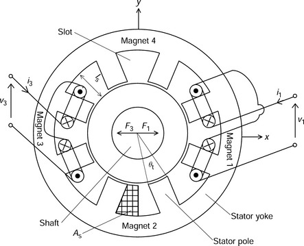
The eight poles are divided into four electromagnets, i.e., magnets numbered 1 to 4. Windings are shown only for magnets 1 and 3. In magnet 1, two short-pitch coils are wound around two stator poles. These coils are connected in series so that only two terminals are required for one magnet. With a current i1 in a coil, MMF, flux and attractive radial force F1 are generated as previously shown in Figure 2.2. Magnet 1 generates radial force in the x-axis direction whereas magnet 3 generates radial force in the opposite (−x-axis) direction. Therefore magnets 1 and 3 are working in differential mode, as previously shown in Figure 2.9. Magnets 2 and 4 produce y-axis radial force also in differential mode.
In the radial magnetic bearing, two perpendicular radial forces, i.e. the x-axis and y-axis forces, are generated. As already mentioned, the four magnets are operating in differential mode with the currents in the four magnets being regulated independently. In total, eight wires are necessary for connection between the radial magnetic bearing and the four current drivers.
Let us define the following parameters:
This means that the area S of one stator pole in airgap is
The radial force F1 generated by two stator poles is derived from (2.25). Since the poles have an angular position of 22.5 deg, the force is:
The self-inductance of one electromagnet with a nominal airgap length of g is
where N is the sum of the number of turns of two short-pitch coils. The radial force can also be obtained from (2.21):
In Figure 2.14 the short-pitch coil on each stator pole has 50 series-connected turns. One turn is composed of two parallel wires, each with a diameter of 0.8 mm. The rated current density in a conductor is 8 A/mm2. The airgap length between the stator pole and rotor surface is 0.4 mm and the slot depth ls is 17 mm. The slot fill factor is defined as the ratio of conductor area to slot area. Find the slot fill factor, the rated current, airgap flux density and radial force of magnet 1 at the rated current. Also find the value of the ratios: radial force/Dl and radial force/rotor weight.
The half slot area As shown in Figure 2.14 is derived by approximating the area as a trapezoid:
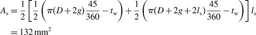
where tw is a tooth width which is given by
The cross-sectional area of the 0.8 mm diameter wire is π × (0.8/2)2 = 0.5mm2. Therefore the conductor area in a half slot is 100 times the cross-sectional area, i.e., 50 mm2. The slot fill factor Sfl is 50/132 = 0.38. The slot fill factor of this short-pitched winding is usually in the range 0.3–0.42 using normal fabrication processes.
The self-inductance is obtained from (2.41). N = 100 turns since there are two coils connected in series, and the inductance is 8.56 mH. The rated current Irt is the product of rated current density, the number of parallel conductors and the conductor cross-sectional area so that Ir = 8A/mm2 × 0.5 mm2 × 2 = 8 A. The flux density at the rated current is Brt = L0Irt/(NS) = 1.26 T and the radial force generated by magnet 1 is given by (2.40) which is calculated to be 632 N.
The radial force density for the rotor shadow area is
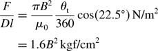
At B = 1.26T, F/(Dl) = 2.6kgf/cm2. The radial force/rotor weight ratio is given by
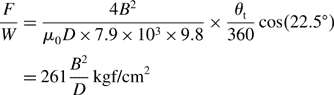
At D = 5 cm and B = 1.26 T, F/W = 83. Note that F/W increases for a small diameter rotor. A small diameter is suited for high acceleration applications.
The derived radial force in this example is about half the value of that in Example 2.8. In Example 2.8, only the magnetic design was considered. However, in Example 2.9, both the magnetic and winding designs are included. For practical radial force limitation and operation, the differentialmode magnetic force should be considered, as shown in the next example.
2.4.1 Linearization
In equations (2.40) and (2.42), radial force is expressed as a function of flux density and current respectively. In order to regulate the radial force the flux density or current should be regulated. Detecting current rather than flux density is advantageous for the following reasons:
1. Current detectors are low cost. These sensors can be installed in current drivers.
2. Flux detection is not easy and can be expensive. One flux detection device is the Hall sensor. The Hall sensor must be extremely thin to be installed in the airgap. Thin Hall sensors are very expensive and mechanically weak. Wiring from the Hall sensor to the controller can also be a problem. Another way to detect the flux is to use search coils. However, dc flux components cannot be detected with search coils.
In most cases, instantaneous current is controlled for radial force regulation. One can see that the relationship between the current and radial force is nonlinear. Without the effect of saturation, the radial force is proportional to the square of the current. In practice, radial force is not proportional to i2, it is rather proportional to i1.6. Let us express the radial forces as
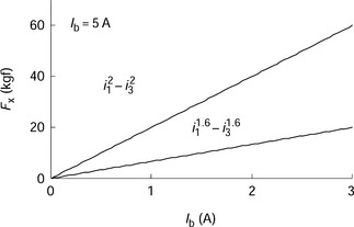
To realize the linear relationships between the radial force and current components, the winding currents in electromagnets 1 and 3 are divided into two current components, i.e., bias current Ib and force regulating current ib:
Note that the currents i1 and i3 are positive values. Hence ib should be less than Ib. The radial force acting on the shaft in x-axis direction is
Substituting (2.44) and (2.45) yields a simple radial force equation
It is now seen that the radial force is proportional to the force regulating current ib when the bias current Ib is kept constant.
Figure 2.15 shows the non-linear characteristics between radial force and winding current for two cases, one is proportional to i2 and another is proportional to i1.6.
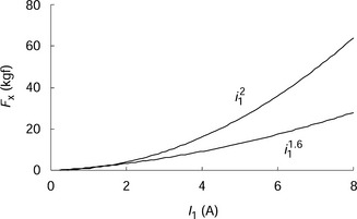
Figure 2.16 shows the relationships between the radial force regulating current component ib and radial force for the above two cases. This confirms that the radial force and ib have a linear relationship as indicated in (2.49). In addition, an almost linear relationship is also obtained for the case where radial force is proportional to i1.6. This numerical result shows the effectiveness of this current component control strategy. One can see that radial force is expressed as
where ki′ = k′iIb and ki is referred to as a force-current factor [1].
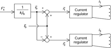
Figure 2.17 shows a block diagram for the current regulation. In the controller, a radial force command F*X and a regulating current component i*b, which is proportional to the force command, are generated. Then the current command is added or subtracted to a constant bias current command I*b based on (2.46) and (2.47). Winding current commands I*1 and I*3 are fed to the current regulators which regulate winding currents to follow these commands. Therefore the sum of generated radial force in electromagnets 1 and 3 will follow the radial force reference F*X.
Find the force-current factor in the 8-pole radial magnetic bearing for the bias current Ib = 4 A. Find the radial forces generated by electromagnets 1 and 3 for ib = 4A at x = 0 and also find the total radial force in the x direction.
The force-current factor is given by
The total radial force is given as a product of ki and ib, which yields 632 N. The radial forces produced by magnets 1 and 3 are
The calculated results indicate the fact that magnet 1 is generating an x-direction radial force of 632 N, while magnet 3 is generating a radial force of 0 N.
2.5 Unbalance pull force
The principles, analysis and examples of unbalance pull force (sometimes called unbalanced magnetic pull) are put forward and discussed in this section. The unbalance pull force is important because it is the cause of inherently unstable characteristics for magnetic suspension systems. The principles are illustrated using a simple example, and then the analysis, including derivation of the unbalance pull force, is introduced. The result is applied to the 8-pole radial force magnetic bearing from the previous section.
2.5.1 Principles
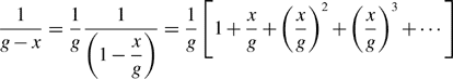
Figure 2.18(a,b) shows simple C- and I-cores with windings. Let us suppose that the winding currents are constant. Note that only the airgap length is different in these figures. In Figure 2.18(a) the nominal airgap length is g, however, in Figure 2.18(b) the airgap length is smaller, i.e., g − x. Let us define Ba and Bb as airgap flux densities in Figure 2.18(a,b) respectively. The flux density in Figure 2.18(b) is high so that Ba < Bb. Therefore the attractive magnetic force between C- and I-cores is high in Figure 2.18(b) since Fa < Fb. Hence the magnetic force is increased when the airgap length is decreased. This characteristic causes the unstable mechanism described below.
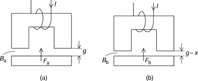
Figure 2.18 Magnetic attractive force and airgap length: (a) wide airgap length; (b) decreased airgap length
If the I-core can be moved in the x direction then it is attracted to the C-core due to the magnetic force. Hence the airgap length decreases. However, this causes the magnetic force to increase. Further movement will only be limited by the two cores becoming clamped together by the force. Therefore the above mechanism is an inherently unstable negative spring system. Hence the magnetic force generated as a function of x is an unstable force. In a successful magnetic suspension system the unstable force should be cancelled by a negative feedback force.
In the case of the differential actuator shown in Figures 2.9 and 2.14, the unstable magnetic force is balanced at the centre position. If a suspended object is moved from the centre position, an unstable magnetic force is generated. The unstable force is a function of eccentric position of a suspended object, so the magnetic force is called an unbalance pull force.
2.5.2 Analysis in C- and I-cores
The principles of unstable force suggest that it is not only a function of current but also a function of displacement x. In the previous sections radial force was expressed as a function of current only and it was assumed that x = 0. However, it is important to include the influence of x.
In section 2.2 an approximation was applied in a mathematical expansion. However, 1/(g − x) can be expanded to include further terms
In sections 2.2 to 2.4, only the first and the second terms in the brackets were considered. The unstable force originates from the third or higher terms. Let us consider up to the third bracketed term. The self-inductance L is
Therefore the stored magnetic energy is written as
Hence the radial force is obtained from the partial derivative of the stored magnetic energy, assuming magnetically linear material, so that
The second term is the unstable force which is a function of displacement x.
2.5.3 Analysis in radial magnetic bearing
Let us define x as a displacement of the rotor from the stator centre position. The unstable force generated by electromagnet 1 in Figure 2.14 is
For electromagnet 3, the same amount of radial force is also generated; however, the definition of displacement and direction of radial force is opposite, so the total unstable force in x-axis is twice that of (2.55) since the force increases for one electromagnet and decreases for the other:
If the winding current is almost equal to the bias current Ib then
where
The coefficient kx, as previously mentioned, is called as a force-displacement factor [1]. In radial magnetic bearings, the force-displacement factor is positive. Hence this force makes the magnetic bearing inherently unstable. Therefore there is a requirement to provide enough negative position feedback to cancel the effect of this coefficient; this is shown in a later section.
2.6 Block diagram and mechanical system
In this section, a magnetic bearing is represented in a block diagram as a linear actuator. In addition, the mechanical system, including the mass of a rotor, is represented.
2.6.1 Radial force
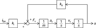
Using the analyses in sections 2.4 and 2.5 the radial force can be derived for the radial magnetic bearing as a function of both the current ib and rotor radial displacement x. The radial force Fx is the sum of these forces
where ibx is the force regulating current in the x-axis. The force-current and force-displacement factors are given by
Figure 2.19 shows a block diagram of (2.59) and the mechanical system. In the block diagram, Fx is a sum of ki ibx and kxx. The radial force is divided by mass m, so that the output of the block is the acceleration ax, which is the input of an integration block. s is the Laplace operator, hence a block 1/s indicates the integration of the input. The integration of acceleration is the radial rotor speed νx. The integration of the speed is the radial displacement x. The mass m is the mass of the suspended object. It can be seen that kx provides a positive feedback loop, which makes the transfer function unstable. A similar block diagram can be drawn for the y-axis variables.
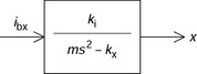
2.6.2 Block diagram
Figure 2.20 shows a simplified block diagram. Now, it is seen that the transfer function is unstable because the denominator (ms2 − kx) is missing a first-order term and includes a negative term −kx. The characteristic equation ms2 − kx = 0 gives
There is a pole in the right half plane so that the transfer function from radial force current component to the radial rotor displacement is unstable. In order to have stable rotor suspension, negative feedback controllers are necessary. In the next chapter, designs of controllers are discussed assuming that the magnetic bearing behaviour is characterized by equation (2.59).