
Mechanical dynamics
An object has six degrees of freedom, i.e., x-, y- and z-axis positions and rotational positions θx, θy, and θz around these three axes. In most magnetic bearing systems, one axis is assigned as the rotating shaft axis so that the rotating shaft should be suspended by active or passive regulation of the remaining five axis positions. Therefore understanding the dynamic constraints of the mechanical system is important.
In this chapter, the dynamic characteristics of a simple mechanical system are described. In the first section, the fundamental equations are described for a two-axis system including the gyroscopic effect. It is important to note that there is cross coupling between axes caused by the gyroscopic effect. Block diagrams provide easy understanding and computer simulations illustrate the system behaviour. In the second section, the two-axis system is extended to four- and five-axis systems. In the last section, a thrust magnetic bearing is described and the requirements for five-axis active suspension are shown.
4.1 Two-axis system
Figure 4.1(a) shows a shaft rotating at an angular speed of ωrm around the k-axis. The three perpendicular x-, y- and z-axes are in the stationary coordinate reference frame. The other three perpendicular i-, j- and k-axes are in the rotational coordinate reference frame. The bottom of the shaft is fixed to the origin of these axes. At a length lrt from the origin, a cylindrical magnetic bearing rotor is fixed to the shaft. Under normal conditions, the k- and z-axes are almost aligned; however, there is always a slight difference. Figure 4.1(b,c) shows the difference. In Figure 4.1(b), a view along the y-axis is shown. The k-axis is inclined by an angular position θy from the z-axis. A moment (or torque) Ny is applied around the y-axis. Note that the angular position and moment are defined around the y-axis using the right-hand rule. In Figure 4.1(c), a view along the x-axis is shown. The angular position and the moment are also defined as θx and Nx respectively, again, based on the right-hand rule.
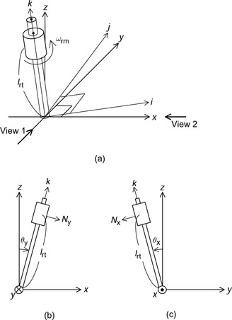
Let us define inertia Ii and Ik around i- and k-axis rotations respectively. The inertia on the j-axis is equal to that on the i-axis because of the symmetrical shaft structure. The product of the inertia and the second-order differential of the angular position with respect to time is equal to the moments so that
The first terms on the right-hand side of these equations are moments originated from the gyroscopic effect. The gyroscopic moment is a product of a z-axis rotational speed ωrm, the k-axis inertia and the angular speed of the perpendicular axis. These terms are effective at a high rotational speed and also with high k-axis inertia such as in a disc-shaped rotor.
Displacements from the cylindrical rotor centre alignment on the x- and y-axes can be obtained from Figure 4.1(b,c); assuming that the inclination of the rotating shaft is small, then
Note that x and y are proportional to each other’s angular positions θy and θx. Solving these equations for θx and θy and substituting into (4.1) and (4.2) yields equations (4.5) and (4.6):
Figure 4.2(a) shows a block diagram for these equations. Acceleration in y-axis is the sum of the gyroscopic term of x-axis speed and the moment term around the x-axis. The gyroscopic term is proportional to the ratio of inertias in the k- and i-axes. Therefore the gyroscopic effect is more substantial for the case of a disc-like shaft rather than a long and thin shaft.
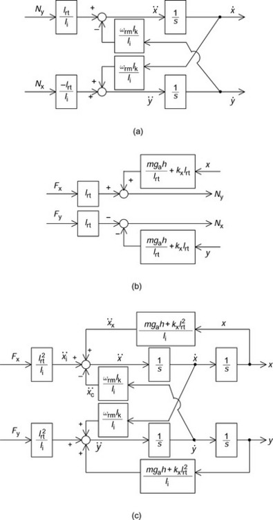
Figure 4.2 Radial force and displacement blocks: (a) torque and speed block diagram (b) the moments Nx and Ny around x- and y-axes (c) radial force and displacement blocks
Next, let us examine the external moment. Suppose that the centre of gravity of a magnetic bearing rotor has a height of h and a mass of m (kg). Note that lrt is equal to h in the ideal case; however, in practice, the sensor target and shaft weight will also have to be considered. Let us define the gravity acceleration as ga. Therefore the moments Nxg and Nyg, around the x- and y-axes, due to the mass, are written as
Let us define the current-driven radial forces, generated in the magnetic bearing on the x- and y-axes, as Fx and Fy. Therefore the moments Nxi and Nyi are generated by currents and given by Nxi = − Fylrt and Nyi = Fxlrt. In addition to the current-driven radial forces, displacement-caused radial forces are also produced. The radial force in y-axis is written as kxy with a force-displacement factor kx and y-axis shaft displacement y. The displacement-originated moment Nxd around the x-axis is written as Nxd = − kxylrt and the moment Nyd around the y-axis is given as Nyd = kxxlrt.
The sum of moments around the x- and y-axes are
Figure 4.2(b) shows a block diagram for the moments. The input variables are current-driven radial forces from the magnetic bearing and also forces from the rotor radial displacement. Radial forces caused by gravity and displacement are generated as a function of the rotor radial displacement. The outputs are the moments around the x- and y-axes. This block diagram can be merged with the previous block diagram.
The moment equations above are substituted into (4.5) and (4.6) to obtain dynamic motion equations such that
Figure 4.2(c) shows the block diagram. The inputs are the suspension radial forces Fx and Fy and the outputs are the x- and y-axis shaft displacements. There are cross-coupling blocks caused by gyroscopic effects and positive feedback loops are caused by weight and the force-displacement factor. This block diagram provides the mechanical system dynamic response.
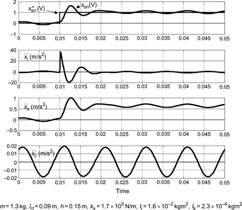
Figure 4.3 shows the waveforms from a computer simulation of the block diagram where a step change in displacement reference in x-axis is applied. Feedback controller blocks have been added and a mechanical unbalance force is considered. The rotational part is made up of a cylindrical rotor with a diameter of 5 cm and a thickness of 3 cm and an additional cylindrical iron part is also included to model the sensor target. The shaft length is about 20 cm long and it is assumed to be of a small diameter and long axial length. The figure shows the x-axis position command x*sn, the radial sensor output xsn, the current-originated acceleration ![]() , the displacement-originated acceleration
, the displacement-originated acceleration ![]() and the gyroscopic acceleration
and the gyroscopic acceleration ![]() . As seen from the figure, the current-originated acceleration is dominant, which is generated by the error between x*sn and xsn. Also, the displacement-originated acceleration is similar in shape to the xsn characteristic, although the peak amplitude is small. The gyroscopic acceleration is almost a sinusoidal function. This is because the radial speed has a variation caused by the mechanical shaft unbalance. In this example, the amplitude is negligible at a speed of 6000 r/min; however, the influence increases with rotational speed.
. As seen from the figure, the current-originated acceleration is dominant, which is generated by the error between x*sn and xsn. Also, the displacement-originated acceleration is similar in shape to the xsn characteristic, although the peak amplitude is small. The gyroscopic acceleration is almost a sinusoidal function. This is because the radial speed has a variation caused by the mechanical shaft unbalance. In this example, the amplitude is negligible at a speed of 6000 r/min; however, the influence increases with rotational speed.
4.2 Four-axis and five-axis systems
In the previous section, the dynamic behaviour of a magnetically suspended machine with two axes of freedom is explained. Based on the equations and block diagrams, dynamic representations of systems with four-axis and five-axis degrees of freedom are described in this section. A simple rigid rotor is considered with a symmetrical structure with respect to the centre of gravity so that the interference between translational and inclination forces can be neglected. Details on rigid and elastic rotor dynamics can be found in References [1,2].
4.2.1 Equation of motion
Figure 4.4(a) shows a shaft with a five-axis active suspension system. There are two radial magnetic bearings and one thrust magnetic bearing. The first radial magnetic bearing, numbered 1, generates radial forces in x1- and y1-axis directions. The second radial magnetic bearing, numbered 2, generates radial forces in x2- and y2-axis directions. A thrust magnetic bearing generates a z-axis suspension force.
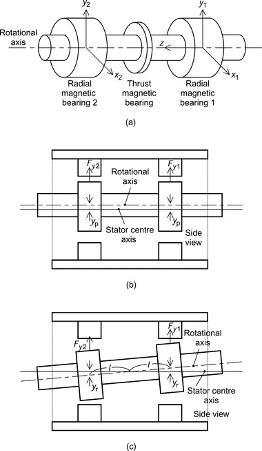
Figure 4.4 Five-axis active positioning: (a) five-axis active positioning; (b) translational displacement; (c) inclination displacement
The radial shaft movements can be expressed by translational and inclination movements. Figure 4.4(b,c) shows these shaft movements. In the translational displacement, the shaft rotational axis is moved in parallel to the stator centre axis. In the example figure, both the rotors are moved by yp in the y-axis direction. In the Figure 4.4(c), a rotor shaft is rotated on the y-axis and rotors 1 and 2 are displaced by yr and − yr, respectively. In the inclination displacement, the shaft rotational axis is rotated with respect to the stator axial centre.
The rotor radial movement is expressed by translational and inclination displacements so that

The translational and inclination forces can be expressed in terms of the radial forces of the magnetic bearings as
The dynamic motion equations for the translational movement have to consider the fact that the radial force is generated by both magnetic bearings. Hence
Note that the gravity force of the shaft weight m is applied in the negative direction of the y-axis. The yp block surrounded by the dotted lines in Figure 4.5 shows the above relationship on the y-axis. The input and output variables are the translational radial force and the displacement.
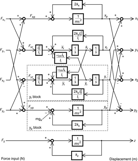
For inclination movement, the dynamic equations in the previous section illustrate that a shaft inclined at an angle given by yr/lrt has an inclination angular acceleration given by ÿr/lrt. The external moment is a sum of current- and displacement-originated terms, i.e., Fyr lrt and (2kxyr)lrt. Therefore the dynamic motion equations are
where Ii and Ik are the inertias around the x- and z-axes respectively. The yr block, surrounded by the dotted lines in Figure 4.5, models the y-axis inclination motion equation. The input variables are the force and x-axis speed, while the output variable is the y-axis movement. This block diagram can be understood with reference to the block diagram in Figure 4.2 from the previous section.
Figure 4.5 shows a block diagram of both the x- and y-axis variables for translational and inclination movement. The radial forces applied to the magnetic bearing rotors are input variables. These variables are transformed into translational and inclination forces using (4.14). Therefore, from these forces, the displacements are obtained using (4.15–4.18). The displacements are transformed into rotor movement using (4.13). In addition to the 4-axis motion equation, a thrust bearing block diagram is added to the bottom of the block diagram. Note that, for simplicity, the thrust movement is taken to be independent of the other axes. The block diagram has force inputs and displacement outputs and it describes the constraints governing shaft motion.
4.2.2 Controller structures
A simple controller structure has independent controls for each axis. Shaft displacements x1, y1, x2 and y2 are detected by displacement sensors and then amplified by controller Gc to generate radial force commands. These radial force commands produce current signals that generate radial forces Fx1, Fy1, Fx2 and Fy2 on the magnetic bearing rotor. The controllers for all axes are independently generating radial force commands.
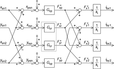
If the gyroscopic effect, or any other interference in x- and y-axes, is considered, then controllers should be designed for the translational and inclination axes. Figure 4.6 shows a block diagram. From the detected shaft movement, displacements on the translational and inclination axes are calculated. These displacements xpsn, xrsn, yrsn and ypsn are then amplified by radial position controllers Gcp and Gcr to produce the radial force reference commands F*xp, F*xr, F*yr and F*yp. From these commands the required radial force commands for magnetic bearings on the x- and y-axes are calculated, so that currents can be supplied to produce the actual radial forces that follow the references. The inclination position block (surrounded by the dotted line) can be improved with additional cross-coupling blocks so that the two-axis interference is cancelled.
4.3 Thrust magnetic bearing and requirement of five-axis suspension
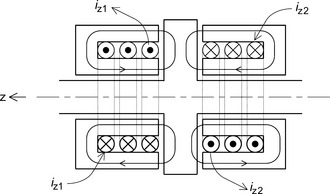
Figure 4.7 shows the cross section of a thrust magnetic bearing. The thrust magnetic bearing generates magnetic force in the axial direction. A ferromagnetic plate is attached to the shaft. On both sides of the plate, cylindrical electromagnets are located so that attractive magnetic forces are generated. The currents iz1 and iz2, produce magnetic forces in opposite directions. These current values are adjusted so that the required magnetic force is generated from the difference of these attractive forces.
The magnetic bearing currents are obtained from the sum of bias and force currents so that
And the axial magnetic Fz force is written as
Therefore the axial force is proportional to the current iz. Hence an axial positioning system can be constructed as follows: using the axial position of the shaft, an axial force command is generated by a controller which produces a current command i*z to control the winding currents iz1 and iz2 that are supplied by inverters.
4.3.2 Requirement of five-axis suspension
Table 4.1 compares inverter and wiring requirements between magnetic bearing and bearingless motor systems with five-axis magnetic suspension. In five-axis active suspension using magnetic bearings, five displacement sensors are required for detection of the shaft positions xsn1, ysn1, xsn2, ysn2 and z. Two radial magnetic bearings and one thrust magnetic bearing are needed. Since magnetic force regulation in one axis requires two single-phase inverters because of the push-pull operation of the magnetic forces, a total of 10 single-phase inverters are required. Therefore 20 wires are needed between the magnetic bearings and inverters. In addition to the magnetic bearings, the motor needs one 3-phase inverter and three wires.
Table 4.1
Comparison of five-axis active suspension
| Magnetic bearing with a motor drive | ||
| Displacement sensors | 5 | xsn1, ysn1, xsn2, ysn2, z |
| Magnetic bearing inverters | 10 | Two single-phase inverters for one axis |
| Magnetic bearing power wires | 20 | |
| Motor inverter | 1 | |
| Motor inverter wires | 3 | |
| Bearingless motor | ||
| Displacement sensors | 5 | xsn1, ysn1, xsn2, ysn2, z |
| Magnetic bearing inverters | 2+2 | Two 3-phase inverters and two single-phase inverters |
| Magnetic bearing power wires | 10 | |
| Motor inverter | 1 | |
| Motor inverter wires | 3 |
In a bearingless motor with five-axis active suspension, the requirements are shown in the bottom half of Table 4.1. For the magnetic suspension, two 3-phase inverters and two single-phase inverters are needed. Two radial-axis positions can be regulated by one 3-phase inverter so four radial-axis positions require two 3-phase inverters with six wires. In addition, two single-phase inverters with four wires are required for a thrust magnetic bearing. Therefore in total 10 wires are required. In addition to the suspension, a 3-phase inverter with three wires is required for the motor drive. The motor windings of two tandem bearingless motor units can be connected in series. One can see that there is a more simple power electronic and wire requirement for a bearingless drive.
The above comparison is based on a bearingless motor with 4-pole and 2-pole windings. In some winding configurations, the requirements may be greater.