
Displacement sensors and sensorless operation
In active magnetic suspension, displacement sensors are necessary to detect the radial (and sometimes axial) movement of the suspended object. Reducing the cost of the sensor is important in developing a bearingless drive since these can be expensive. Hence practical problems and solutions concerning sensor development are described in this chapter. The requirements for a displacement sensor can be summarized as follows:
(a) Wide frequency response – The frequency response bandwidth should be high enough so that the phase margin of the magnetic suspension loops does not need to be decreased. For example, if the cross-over frequency of a magnetic suspension loop is 100 Hz then the sensor response should be more than 5 kHz.
(b) Low noise – If there are high frequency noise components then these will be amplified by the derivative operation of a PID controller so that there will be significant noise in the suspension force references. If this occurs then the suspension current commands also include significant noise leading to current regulator saturation for a short time. This saturation results in a serious delay in the magnetic suspension loops which may cause shaft touch-downs in the stator bore.
(c) Low interference noise – In some displacement sensors, interference noise is generated if two or more sensors are installed. This is usually the case in order to detect x- and y-axis displacements. The sensor interference can take the form of a signal with a voltage of a few mV and a frequency of a few kHz. This can be a significant problem as described in (b) above.
In addition to the above requirements, low temperature drift, good linearity, compactness, as well as reliability are required.
In the first section of this chapter, the principles and problems of a displacement sensor with a magnetic core and winding are discussed. In the second section some methods to improve sensor performance are described, and a performance comparison of the inductive and eddy current types of sensor is put forward. In the third section the problems associated with a rotating target is highlighted. In the final section the sensorless displacement operation of a bearingless motor is introduced.
18.1 Principles of displacement sensor
Displacement sensors detect the linear position during the movement of an object without a mechanical contact. To the author’s best knowledge these devices take the form of three basic types: capacitive, laser and electromagnetic. In capacitive sensors, the airgap length is detected using a variation in capacitance. Therefore good isolation between the sensor and the shaft is necessary. In addition, the air must be clean and oil and other particles should not be present because this will affect the dielectric. In laser sensors, displacement is detected by reflected laser light so that a uniform target surface is required to prevent noise. These sensors can be used, in some cases, in a bearingless motor application; however, electromagnetic sensors are still considered better for general-purpose applications. Therefore electromagnetic sensors are described in the following sections since they are the usual type of device used in bearingless drives.
Figure 18.1 shows the structure and principle of operation of an electromagnetic displacement sensor. An E-shaped magnetic core has a winding with two terminals. A target (rotor shaft) is drawn as a rectangular solid having airgap length of lg. The input impedance at the terminals varies with the airgap length. If the input terminals are excited by a high frequency voltage then the coil impedance will be dominated by the inductance (which is the variable part of the impedance) and it is obtained by detecting the terminal voltage and current.
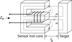
There are two types of electromagnetic sensors. One is inductive while the other is an eddy current type. In inductive sensors, the target is made of a ferromagnetic material of high permeability such as laminated silicon steel, ferrite and carbon steel. The excitation voltage frequency is in the range of 20–100 kHz and the inductance varies as a function of airgap length (approximately inversely). If the airgap length is small then there is high impedance.
In eddy current sensors, the target is made of a conductive material of low resistance such as copper, non-magnetic stainless steel, aluminium, carbon steel and other metallic material. The excitation voltage frequency is high, for an example 2 MHz, so that eddy currents are generated in the target. If the target is close to the sensor core then eddy currents are induced into the target which reduces the flux (almost as a short-circuit transformer) and produces a low input impedance. As the target moves away, the coupling decreases which increases the input impedance (which is opposite to the inductive type).
Figure 18.2 shows current variation with respect to the airgap length for different target materials; the iron core of the sensor is ferrite which has good permeability at 400 kHz and it takes the form of a cylindrical pot core with an outer diameter of 3.3 mm. The target materials are copper, aluminium, carbon steel and ferrite. The carbon steel is referred to as iron in the following sections. The terminal voltage is constant. The following characteristics can be observed:
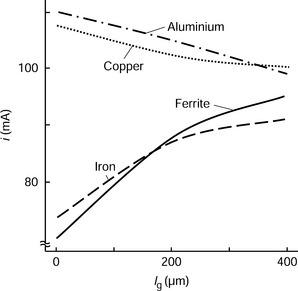
Figure 18.2 Sensor current and airgap length with several target materials at 400 kHz with a ferrite core
(a) The winding current increases with airgap length when the iron and ferrite targets are used because these materials have high permeability so that the inductance decreases with increasing airgap length.
(b) On the other hand the winding current decreases when the aluminium and copper targets are used because these materials have low resistance and allow eddy current flow.
(c) For the iron and ferrite targets the current is significant even when the airgap length is zero. This is because the magnetic reluctance in the iron core is finite so that it is not dominated by the reluctance of the airgap alone.
(d) For all materials the current variation with respect to the airgap length is only 10 to 20% of the maximum line current. Hence the sensitivity of winding current to airgap length variation is not very good.
(e) In all cases the current variation becomes saturated with a large airgap length because the input impedance becomes dominated by inductance due to the leakage fluxes Ψ1.
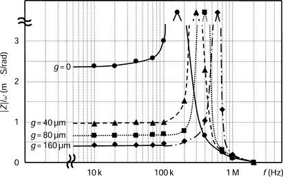
Next let us look at the case when laminated silicon steel is employed as the excitation core [1]. Figure 18.3 shows the frequency characteristics for the input impedance of a bearingless motor winding with a laminated silicon steel core. This is the standard material in electrical machines (as opposed to small ferrite actuator cores) because manufacturing is straightforward; however, its high frequency characteristics are not as good as for ferrite material. Three different curves are drawn using the measured points and assumed equivalent circuits. Curve 1 is obtained by assuming that the iron permeability is infinite and there are no iron losses although there is stray capacitance. The stray capacitance exists between the turns of the winding so that the equivalent circuit is drawn with a parallel capacitance across the winding inductance. Hence a resonance is seen at 700 kHz. Curve 2 is obtained by considering iron loss in the silicon steel core so that an iron loss resistance is placed in parallel with the inductance. The resistance value is a function of the excitation frequency, and the impedance decreases at high frequency. Also the phase angle is less than 90 deg (since it is an RL circuit), which more closely matches the measured input impedance. Curve 3 is similar to curve 2 except there is now a decrease in permeability of the core due to high frequency, therefore producing a better correspondence with the measured results.
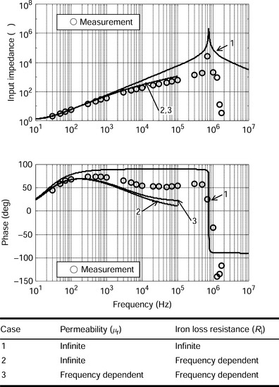
Figure 18.3 Frequency dependence of input impedance for a sensor winding in silicon steel with influence of permeability decrease and iron loss
From this figure the following observations about silicon steel displacement sensors can be made:
(a) The excitation frequency should be less than the resonant frequency.
(b) Core loss is not negligible in silicon steel at a frequency of more than 1 kHz.
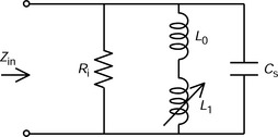
Figure 18.4 shows the equivalent circuit of a sensor winding. The inductance L0 is constant while the inductance L1 is the airgap-length-dependent-inductance. Cs is the stray capacitance and Ri is the iron loss resistance. Hence this circuit includes all the characteristics exhibited in curves 1–3 in Figure 18.3.
18.2 Improvements in sensitivity
As shown in the previous section, the current variation with respect to the airgap length is less than 20% of the winding current. The airgap length is detected as a function of current so that sensitivity improvement is necessary. In this section, two methods are introduced. One is a resonant circuit and the other is a differential circuit.
18.2.1 Resonant circuit
Small variations in the sensor inductance can be amplified with a resonant circuit. This can be simply constructed with an external capacitance connected in parallel to the sensor winding terminals.
Figure 18.5 shows an example of the input impedance variation for several airgap lengths. A parallel capacitance is connected. When an airgap length is zero, the inductance value is high so that the resonant frequency, i.e., ![]() , is low. At this resonant frequency, the input impedance is maximum, and as the airgap length increases so does the resonant frequency.
, is low. At this resonant frequency, the input impedance is maximum, and as the airgap length increases so does the resonant frequency.
One way to take an advantage of the resonance is to set the excitation frequency to around 200 kHz giving an improved input impedance variation. This is detected by voltage or current amplitude variation (when using a current- or voltage-sourced supply). The amplitude can be transformed into a dc voltage in several different ways. The complete circuit can be realized using operational amplifiers, multiplier devices and rms-to-dc converter ICs. Another way is to track the resonant frequency with an oscillating circuit where the oscillating frequency indicates the airgap length.
18.2.2 Differential circuit
Figure 18.6(a,b) shows the magnetic and electric circuit arrangement for a differential type of displacement sensor. There are two E-shaped cores. Core 1 faces a target with a variable airgap lg while core 2 faces a fixed target. Two isolated windings (1 and 2) are wound on the cores. Winding 1 carries the excitation current while winding 2 detects the core flux in each core. Figure 18.6(b) shows the circuit connection. The two coils of winding 1 are connected in series and excited by a voltage source v0. The two coils of winding 2 are also connected in series but one has reversed polarity so that the induced voltages v1 and v2 in winding 2 are subtracted at the output terminals so that v3 = v1 – v2. If the airgap length lg is equal to the airgap of the fixed target then the output voltage is zero. Hence the output voltage varies as a function of the airgap length of the moving target and can be set to zero when the fixed target airgap is equal to lg for the case of a centred rotor. The ac output voltage can be transformed into dc as described above.
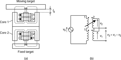
Figure 18.6 Differential sensor structure and principles: (a) iron core and winding arrangement; (b) circuit connection
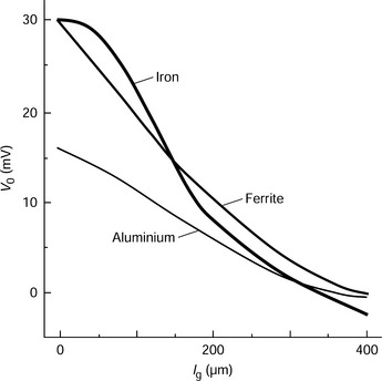
Figure 18.7 shows the output voltage characteristics for a differential sensor with several different target materials. Note that the airgap length of the fixed target is set to about 400 μm. The sensor core is made from ferrite material with an excitation frequency of 400 kHz. A comparison with Figure 18.2 shows that the output voltage has a wider variation with respect to the airgap length. However, linearity still remains a problem but a microprocessor can be used to produce a linear characteristic via a look-up table or some other technique.
18.3 Inductive and eddy current sensors
One of the problems of a displacement sensor is associated with the surface quality of the rotating target ring. Since the displacement sensors detect the airgap length using the rotating shaft, the shaft surface may not be uniform and small cracks and scratches may be present. This is particularly relevant to eddy current sensors where a small mechanical crack may prevent the induced eddy currents, so errors will occur.
Figure 18.8 shows the sensor output waveforms for sensors along two perpendicular axes. The shaft is not rotating but reciprocally vibrating. The waveforms of xE and yE are the output voltages from eddy current sensors while xI and yI are the output voltages from inductive sensors. These sensors are adjacent to each other and measuring the same vibration, and the shaft is vibrating in a sinusoidal manner at 100 Hz by magnetic forces applied in the x- and y-directions. It can be seen that the output voltages of both the eddy current and the inductive sensors correspond.
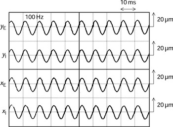
Figure 18.9 shows the same output waveforms with the rotor rotating at 100 r/s. A mechanical unbalance causes a rotating vibration as seen in the output voltages of the inductive sensors. A similar vibration is seen in the eddy current sensor outputs; however, there are also high frequency components in the waveforms. This noise is caused by surface imperfections in the rotating target ring. The inductive sensors are not as sensitive as the eddy current sensors for the following reasons:
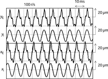
(a) The excitation frequency of an inductive sensor is low, so the sensor magnetic pole area is large. If the pole cross section is large then small target cracks have a negligible effect. However, small poles are required in eddy current sensors to minimize stray capacitance.
(b) The inductive sensor can be made from laminated silicon steel so that several magnetic poles can be situated around the circumference (like a motor stator). In this case the differential voltages detected in opposite magnetic poles, as well as neighbouring poles, can be processed. The signal processing eliminates the second-, third- and higher-order harmonics caused by deformation and imperfections in the target ring.
When comparing the figures, the advantages of the inductive type of sensor are obvious. However, there are disadvantages with inductive sensors as listed below:
(a) There are few, if any, inductive sensors available on the market.
(b) The shaft target ring has to be made from laminated silicon steel.
(c) The excitation frequency is low, so the filtering of the carrier frequency component may cause a delay in the sensor response.
In eddy current sensors, further improvements of the output voltage are possible:
(a) Two eddy current sensors can be placed on one axis and the output voltages are subtracted to give differential operation. The second harmonic and even harmonics are reduced and temperature drift is decreased.
(b) The target material can be replaced with non-magnetic stainless steel to avoid magnetic imperfections. Also copper can be used in some applications. In these cases, adjustment for the nonlinear characteristics should be made in the sensor amplifier.
(c) The sensor head diameter should be small so that the target ring does not interfere with the two-axis movement. For example, the sensor head diameter should be 5 mm or less for a target ring diameter of 50 mm. On the other hand, the sensor head diameter should be large compared to the airgap length for better sensitivity and linearity. For example, a head diameter of 5 mm should be used for 1 mm airgap length or less.
(d) The excitation frequency of the x-, y- and z-axis sensors should be set far enough apart to avoid interference with each other. The difference in excitation frequencies should be greater than the frequency range of the sensor. For example, for a sensor response range of 20 kHz, when the x-axis sensor is excited at 2 MHz the frequencies of the other sensors should be less than 1.96 MHz or higher than 2.04 MHz to provide enough frequency separation.
18.4 Sensorless bearingless motor
If the shaft displacement can be estimated or calculated from the terminal voltage and current then the shaft structure can be simplified and shortened because the sensor target rings are not needed. In addition, assembly, installation and resonant vibration problems associated with flexible shafts can be avoided. Many different ways to remove the position sensors in magnetic bearings have been investigated and these can be split up into the following categories:
(a) High frequency sinusoidal current injection [2].
(b) PWM carrier injection [3–6].
(d) Observer-based calculation [7].
These methods can also be applied to the bearingless machine.
Method (a) is similar, in principle, to the inductive displacement sensor. High frequency sinusoidal voltages and currents are injected and the impedances or induced voltages are detected to estimate the shaft displacement. The injected frequency is sufficiently high so that it does not interfere with the motor and suspension currents. However, the precision may be inferior to that of the inductive sensor because the motor and suspension fluxes are dominant and may interfere with the injected high frequency component. In order to inject the carrier signal, an analogue power amplifier, suitable for low power applications, can be used. However, for fractional horse-power applications, a PWM inverter should be used instead – in which case, the PWM carrier frequency has to be high enough to inject the sinusoidal component.
Method (b) is similar to (a); however, the PWM carrier signals are used for the displacement estimation. Modern PWM inverters are low cost and compact and also have high efficiency and low losses.
Method (c) uses flux detectors similar to Hall probes. If the rotor shaft is displaced from the stator centre then the flux distribution becomes unsymmetrical. The rotor shaft position is then estimated from the flux unbalance.
Method (d) estimates the rotor radial position from the terminal voltage and current using a mathematical electromagnetic representation. The dynamic radial position is obtained by an observer although the absolute position, i.e., the radial position at low frequency, is missing. Inductance and resistance parameters have to be obtained over wide frequency and current ranges to implement the strategy.
A combination of the above position-sensing techniques is possible.
In this section, method (a) is briefly described [8] where a high-frequency current is injected into the motor windings and detected in the suspension windings. Let us suppose that ima and imb are the instantaneous 2-phase high-frequency currents in the motor windings. Let us also suppose that the suspension current can be neglected because it is at a substantially lower frequency. Therefore the flux linkages λsa and λsb of the suspension windings can be written as
where M′ is constant (M′ is the derivative of mutual inductance with respect to the rotor radial position) and x and y are the radial positions of the rotor in two perpendicular radial axes. This equation indicates that the mutual coupling between the motor winding and the suspension winding is proportional to the radial displacement of the rotor.
Let us only look at the high frequency current component, at an angular frequency of ωh, which is generated in the ma-phase of the motor winding. Neglecting the low frequency torque and suspension current, the motor current simplifies to:
where I4 is the rms value of the injected high frequency current.
Substituting (18.2) into (18.1) and executing the derivative of the flux linkage, the voltages vsa and vsb, at the suspension winding terminals, are obtained:
The derivatives of the radial positions are normally small compared to the product of the radial position and ωh so that the induced voltages at the suspension winding terminals can be simplified to
This equation indicates that high frequency voltages are induced into the suspension windings and these have amplitudes that are proportional to the rotor radial displacement. Therefore the signal processing of these induced voltages will provide the rotor displacement information.
Figure 18.10 shows the relationship between the induced voltage and the rotor radial displacement x. It can be seen that the induced voltage is almost proportional to the displacement. Also note that the differential voltage principle, as described in the previous section, is an inherent characteristic in this case because the 4-pole and 2-pole windings are employed and the mutual inductance between the two is zero at the centre position. There is also a good range of voltage variation as a function of the radial displacement. The measurements were carried out over a range of frequencies. At 20 kHz the voltage gain (2.56 mV/μm) is about one-tenth of that at 50 Hz when a conventional iron core of laminated silicon steel is utilized. The reduction of permeability and the iron loss are the causes of the reduced voltage gain at a high frequency.

Figure 18.11 shows a block diagram of the displacement sensing circuit. The terminal voltages vsa and vsb are detected and fed to a band-pass-filter (BPF) circuit to obtain the carrier frequency component and eliminating other frequency components (such as the main suspension winding frequency and the motor revolving field components); these signals are then multiplied by a carrier frequency for demodulation. The low-pass-filter (LPF) eliminates the high frequency component (which has twice the carrier frequency) to obtain dc values so that the estimated displacements xe and ye are proportional to the rotor displacement.
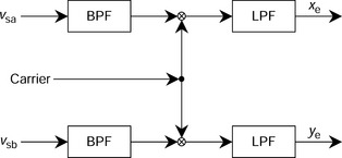
Figure 18.12 shows a spectrum of the suspension winding terminal voltage. It can be noted that the carrier frequency is set to 20 kHz, and the main suspension voltage components are below several kHz.
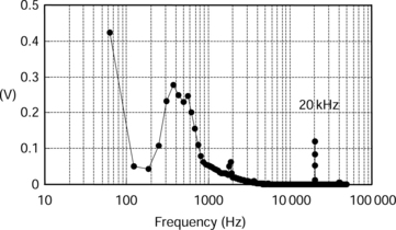
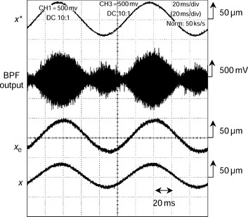
Figure 18.13 shows the operating waveforms when the radial position command x* is intentionally varied in a sinusoidal manner. The BPF output signal amplitude is almost proportional to the radial displacement. The estimated displacement xe and the detected displacement x (as detected by an eddy current sensor) are shown and good correlation is seen.
The estimated radial position was used in the radial position feedback loop and stable operation was obtained. However, careful gain adjustment in the radial position regulator and a decrease in the current limit of the radial force winding were required because the frequency response of the estimated radial position was inferior to that from the eddy current sensor. Despite the relatively low stiffness of the radial suspension, a low cost and compact bearingless motor drive can be realized.
References
[1] Kuwajima, T., Nobe, T., Ebara, K., Chiba, A., Fukao, T., “An Estimation of the Rotor Displacements of Bearingless Motors Based on a High Frequency Equivalent Circuit”. IEEE PEDS conference Bali, 2001:725–731. [October IEEE Catalogue No. 01TH8594C, ISBN 0-7803-7234-4].
[2] Choi, C., Park, K., “A Sensorless Magnetic Levitation Systems Using a LC Resonant Circuit with PPF Control”. Proc. MOVIC ’98, Vol. 2, Zurich, Switzerland, 1998:739–744. [August].
[3] Mizuno, T., Namiki, H., Araki, K., “Self-sensing Operations of Frequency-Feedback Magnetic Bearings”. Proc. Fifth International Symposium on Magnetic Bearings, Kanazawa Univ., 1996:119–123.
[4] Matsuda, K., Okada, Y., Tani, J., “Self-sensing Magnetic Bearing Using the Principle of Differential Transformer”. Proc. Fifth International Symposium on Magnetic Bearings, Kanazawa Univ., 1996:119–123.
[5] Tsao, P., Sanders, S.R., Risk, G., “A Self-sensing Homoplar Magnetic Bearing: Analysis and Experimental Results”. IEEE IAS 34th Annual Meeting, 1999:2560–2565.
[6] Yoshida, T., Ohniwa, K., Katsuyama, Y., “A Position-Sensorless Magnetic Levitation Control Method”. Proc. IEEJ JIASC 2001, Vol. 271, 2001:1385–1390.(in Japanese)
[7] Mizuno, T., Araki, K., Bleuler, H., “Stability Analysis of Self-sensing Magnetic Bearing Controllers”. IEEE Trans. on Control Systems Technology, Vol. 4, No. 5, 1996:572–576.
[8] Muronoi, K., Andoh, N., Chiba, A., Fukao, T., “Characteristics of Induction type Self-sensing Bearingless Motors”. Proc. IPEC-Tokyo, 2000:2109–2114.