
Primitive model and control strategy of bearingless motors
In this chapter, a primitive bearingless machine is introduced. This machine can generate radial forces so that it can be used as a magnetic bearing; it is used here to illustrate the principles of magnetic suspension in bearingless motors. A typical bearingless stator with 4-pole and 2-pole windings and a cylindrical rotor made of silicon steel are described.
6.1 Principles of radial force generation
Figure 6.1 shows the cross section of a primitive bearingless motor under different conditions. In Figure 6.1(a), there is a symmetrical 4-pole flux distribution. The solid curves illustrate the flux paths circulating around the four conductors 4a, these conductors are located in the stator slots. The 4-pole flux wave Ψ4a produces airgap poles in the order N, S, N and S in the airgap sections 1, 2, 3 and 4 respectively. Since the flux distribution is symmetrical, the flux density magnitudes in airgap sections 1, 2, 3 and 4 are of the same value at the same point in the pole section. There are attractive magnetic forces between the rotor poles and stator iron. The amplitudes of these attractive radial forces are the same, but the directions are equally distributed so that the sum of radial force acting on the rotor is zero.
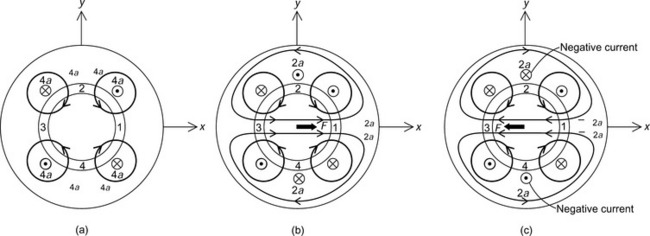
Figure 6.1 Principles of radial force generation: (a) 4-pole symmetrical flux; (b) x-direction radial force; (c) negative x-direction force
Figure 6.1(b) shows the principle of radial force generation. Two conductors 2a are located in the stator slots. With the current direction as shown in the figure, a 2-pole flux wave Ψ2a is generated. In airgap section 1, the flux density is increased because the direction of the 4-pole and 2-pole fluxes is the same. However, in airgap section 3, the flux density is decreased because the direction of these fluxes is opposite. The magnetic forces in the airgap sections 1 and 3 are no longer equal, i.e., the force in airgap 1 is larger than in airgap 3. Hence a radial force F results in the x-axis direction. It follows that the amplitude of the radial force increases as the current value in conductors 2a increases.
Figure 6.1(c) shows how a negative radial force in the x-axis direction is generated. The current in conductors 2a is reversed so that the flux density in airgap section 1 now decreases while that in airgap section 3 increases. Hence the magnetic force in airgap section 3 is larger than that in airgap section 1, producing a radial force in the negative x-axis direction.
Figure 6.2 shows radial force generation in the y-axis direction. Two conductors 2b, which have an MMF centred on the y-axis, are added to the stator. A similar flux density imbalance occurs but this time between airgap sections 4 and 2, hence producing a force on the y-axis. The polarity of the current will dictate the direction of the force.
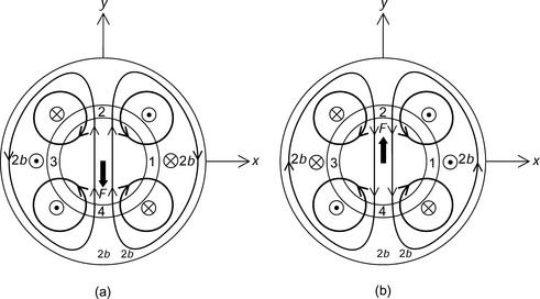
Figure 6.2 y-Direction radial force: (a) negative y-direction radial force; (b) y-direction radial force
These are the principles of radial force generation in x- and y-axis directions. The force values are almost proportional to the current in conductors 2a and 2b (assuming constant 4-pole current). The vector sum of these two perpendicular radial forces can produce a radial force in any desired direction and with any amplitude.
Figure 6.3 shows the flux plots for a primitive bearingless motor. In Figure 6.3(a), a symmetrical 4-pole flux distribution is seen with an excitation of the 4-pole winding. The 4-pole conductors are placed in stator slots as shown. Only the u-phase conductors are shown to represent current density, although the other windings are simultaneously excited using a symmetrical 3-phase current set. In Figure 6.3(b) the 2-pole 3-phase winding is also excited so that the flux distribution is unbalanced, which results in a radial force in the x-axis direction.
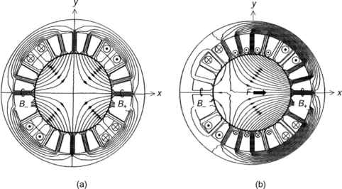
Figure 6.3 Radial force generation in a primitive bearingless motor: (a) symmetrical 4-pole flux distribution; (b) radial force generation
Figure 6.4 shows another example of a surface-mounted permanent magnet (SPM) bearingless motor. The permanent magnets are magnetized to generate a 4-pole flux distribution. In Figure 6.4(a) a symmetrical 4-pole flux distribution is seen. In Figure 6.4(b) the 2-pole winding is excited. With the superimposed 2-pole flux wave, the flux distribution is not symmetrical; the flux density in permanent magnet A is high while in C it is low. Hence a radial force is generated in the x-axis direction.
6.2 Two-pole bearingless motor
In the previous section the 4-pole winding is the main motor winding so that the 2-pole winding is used as the suspension winding in order to generate radial forces. It is possible to change the role of the windings. In this section a bearingless motor with a 2-pole motor winding is shown. This 2-pole configuration is useful in induction type bearingless motors.
Figure 6.5 shows the radial force generation. In Figure 6.5(a) the 2-pole conductors 2a are excited as a motor winding so that a strong 2-pole flux distribution is produced. The 4-pole conductors 4a produce a weak 4-pole flux wave. The flux density in airgap section 1 is increased, but decreased in airgap section 3. Hence radial force is generated in the x-axis direction. Negative-direction radial force can be generated by reversing the current in conductors 4a.
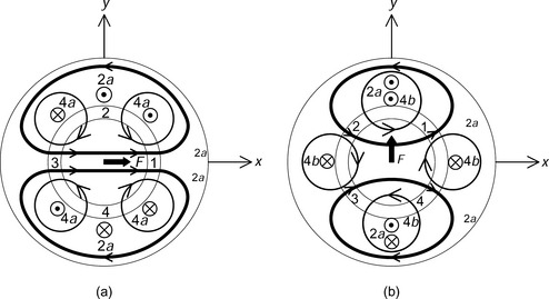
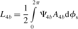
Figure 6.5(b) shows the radial force generation in the y-axis direction. The conductors 4b, which are electrically perpendicular (which is 45 mechanical deg) to conductors 4a, are excited. A 4-pole flux wave is generated. This flux wave is superimposed on the strong motor flux Ψ2a so that the flux density in airgap sections 1′ and 2′ is increased whereas it is decreased in airgap sections 3′ and 4′. Therefore radial force is generated in the y-axis direction; a negative current in conductors 4b will generate negative y-axis radial force.
The flux distribution in Figure 6.5(a) is similar to the one in the previous section (Figure 6.4(a)). The radial force is generated by the flux density variation in the magnetic poles. However, in Figure 6.5(b), the flux distribution is slightly different. The airgap sections 1 ′,2′,3′ and 4′ are not exactly positioned at the centre of the 2-pole flux wave, so if a salient-pole rotor is employed, the generated radial force is reduced in Figure 6.5(b) compared with that in Figure 6.5(a). Hence a 2-pole motor drive is suitable for a machine with a cylindrical rotor, like an induction and SPM machines. In the case of a salient-pole synchronous machine, the unsymmetrical characteristics can be compensated in a decoupling controller, which results in unsymmetrical current injection. The 2-pole drive is also suitable for large airgap structures.
6.3 MMF and permeance
In this section, the MMF of a 2-phase winding is expressed as a sinusoidal function with an approximation to the fundamental component. The permeance variations caused by airgap length variation due to eccentric rotor displacement are derived to provide a basis for inductance-variation and radial-force expressions for use in further sections. The following assumptions are made:
(a) The MMF spatial distribution is approximated to the fundamental component.
(b) Magnetic saturation is neglected.
(c) Airgap permeance distribution is smooth. Stator slot harmonics are neglected. The rotor and stator surfaces are cylindrical and smooth.
(d) The magnetic reluctance of the iron core is negligible. The iron permeability is infinite.
(e) Eccentric rotor displacement is small with respect to the airgap length between the rotor surface and stator inner surface. This displacement is also small compared to the rotor radius.
Figure 6.6 shows the winding arrangement for a primitive bearingless motor. Two sets of 2-phase windings are wound on the stator. The 4-pole windings are 4a and 4b and the 2-pole windings are 2a and 2b. The positive current directions of each winding are shown in the figure. Note that current directions in the 2a and 2b windings are arranged such that the MMF directions are aligned on the x- and y-axis directions respectively. The 4a winding is arranged so that the MMF direction in airgap 1 is also aligned to the x-axis and the 4b winding is arranged to be perpendicular to the 4a winding in electrical terms with a phase-lead angle of 90 electrical deg (45 mechanical deg) in the counter-clockwise direction. If co-sinusoidal and sinusoidal currents, with a frequency of 2f, are supplied to the 4a and 4b windings then a magnetic field, revolving in a counter-clockwise direction with speed f, is generated. For the case of the 2a and 2b windings, with co-sinusoidal and sinusoidal currents with frequency f, the rotational direction is also counter-clockwise with a rotational speed of f. The flux lines show the case for a point in time when there are positive currents in 2a and 4a and zero in 2b and 4b, which results in force in the x-axis.
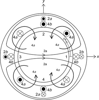
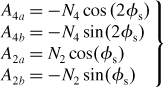
The MMF space distributions for the 4a,4b,2a and 2b windings with unity current can be written as
where N4 and N2 are the amplitudes of the fundamental component of MMF distribution. The angular coordinate φs is a counter-clockwise rotational angular position starting from the x-axis. Note that the positive direction of MMF is defined in the radial direction from the rotor to the stator. For example, a flux Ψ4a generated by a positive dc current in the 4a winding is positive because it flows from the rotor to the stator teeth in airgap section 1, where φs = 0.
Figure 6.7(a) shows a rotor having an eccentric displacement from the stator centre. The perpendicular x- and y-axes are fixed to the stator centre. The rotor centre is displaced in the positive direction along the x- and y-axes. Figure 6.7(b) shows an enlarged figure illustrating the coordinate system. Let us assume that the airgap length between the rotor and stator is g0 when the rotor is centred in the stator bore. If the rotor displacements are x and y then the airgap length g between the rotor and the stator is
The inverse of the airgap length can be written with an assumption that the displacements are small compared to the nominal airgap length g0 so that
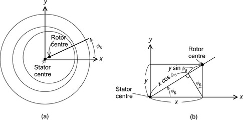
Figure 6.7 Airgap length variation with rotor eccentric displacement: (a) coordinate definition; (b) stator and rotor centres
The permeance P0 at an angular position φs is
where R and l are the rotor radius and axial length.
Figure 6.8 shows an alternative representation of the winding and coordinate arrangement. Note that the polarity of winding 4a is reversed. The definition of the stationary angular position φs is defined in the clockwise direction and the rotor also has clockwise rotation. As shown in Figure 6.6, the x- and y-axes are defined and 2a and 2b are arranged to generate MMF on these axes. Windings 4a and 2a are advanced by 90 electrical deg in the clockwise direction with respect to 4b and 2b. This arrangement of the windings and coordinates will be used in the examples throughout this chapter. Find the equations corresponding to equations (6.1–6.4). Also show the airgap length distribution and permeance.
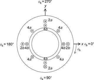
The MMFs for unity current are
The airgap length is written as
Note that the sign of y is positive because the φs direction is reversed. Therefore the permeance distribution is
6.4 Magnetic potential and flux distribution
In this section, the airgap flux distribution is derived using the MMF and permeance distribution. In the calculation process it is quite important to assume that the magnetic potential of the rotor is not zero because flux distribution is unsymmetrical when a rotor has radial displacement.
Figure 6.9 shows a simplified magnetic circuit and the electrical equivalent circuit. In Figure 6.9(a), a cylindrical iron rotor and a surrounding iron stator are shown. On the stator, conductors 2a are located in slots. These conductors are connected in series to form a winding 2a. With unity current in the winding, a sinusoidal space MMF distribution is generated.
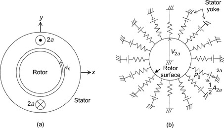
Figure 6.9 Magnetic potential and equivalent circuit: (a) magnetic circuit; (b) equivalent electrical circuit
In Figure 6.9(b), an electrical equivalent circuit is drawn. The conductances represent the airgap permeances given by (6.6). The conductance values are not equal; rather the values are dependent on the rotor radial displacement and angular position φs. In series with the airgap permeances are dc voltage sources. These voltage sources represent the MMF of winding 2a. The voltage values are half of A2a as given in (6.3). The voltage sources are not included at φs = 90 and 270 because A2a is zero. The values of the voltage sources are also dependent on φs. The ground symbols connected to the voltage sources indicate that the stator yoke magnetic potential is assumed to be zero and that the stator tooth and yoke reluctances are also assumed to be zero.
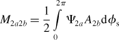
The ring circuit connecting all conductances represents the rotor surface permeance, which is assumed to be infinite. The voltage V2a is the magnetic potential of the rotor. In total, 16 branches of conductances and voltage sources are drawn in the figure to illustrate the calculation concept; however, the mathematical calculation can be processed using a large number of branches since it is really a distributed network. The current values in the branches correspond to the airgap flux. Hence the flux Ψ2a in one branch is written as
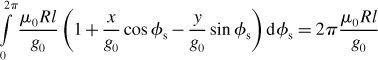
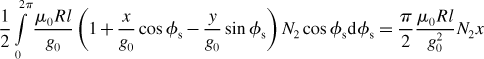
An integral of the flux around the rotor surface should be zero according to Gauss’ law, so the following equation is obtained
Substituting (6.10) into (6.11) and solving for the rotor magnetic potential results in
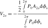
Substituting (6.3) and (6.6) into this equation and solving the integral yields a simplified result for the rotor magnetic potential:
From this equation, we can observe the following:
(a) The magnetic potential is zero if the rotor is positioned at the stator centre.
(b) When the rotor has x-axis displacement, the rotor magnetic potential is proportional to the displacement.
(c) The airgap flux distribution is no longer symmetrical as shown in (6.10).
Note that the rotor magnetic potential calculation is quite important in the analysis of bearingless motors. If zero magnetic potential is assumed as in conventional motor analysis then an unsymmetrical flux distribution is not correctly defined and the radial force calculation is inaccurate.
In a similar manner, a magnetic potential also exists when exciting the winding 2b with unity current:
where the rotor magnetic potential is proportional to the y-axis rotor displacement.
It is possible to derive the magnetic potentials that excite the 4-pole windings 4a and 4b. In these cases the resulting magnetic potential is zero and does not depend on the rotor radial displacement. This can be simply explained by way of example: 2a in (6.12) is substituted by 4a, which is a periodic function of 2φs. The permeance given in (6.6) is a periodic function of φs; therefore the integration of this product is zero.
The airgap flux distributions produced by windings 2a,2b, 4a and 4b when excited by a unity current are
The rotor magnetic potential is not zero when the 2-pole winding is excited with a radial displacement.
Derive rotor magnetic potentials using the alternative coordinates shown in the previous example.
The definition of rotor magnetic potential in (6.12) is not dependent on the winding arrangement and angular position. Thus, the denominator in (6.12) is
Therefore we get exactly the same expression as (6.13) for the rotor magnetic potential. In the calculation of the y-axis rotor potential, the same expression as (6.14) is obtained.
6.5 Inductance matrix
In this section, the inductance matrix is derived using the airgap flux distributions, as found in the previous section. Some elements of the inductance matrix are shown to be a function of the radial rotor displacement.
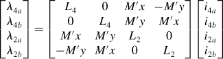
Let us suppose that the flux linkages of windings 4a, 4b, 2a and 2b are λ4a, λ4b, λ2a and λ2b respectively. Let us also suppose that instantaneous currents of windings 4a, 4b, 2a and 2b are i4a, i4b, i2a and i2b respectively. The flux linkage and current relationships are expressed in a matrix form as
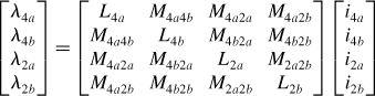
The inductances defined in the above matrix form can be derived by integration of the product of airgap flux and winding distribution such that
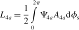
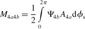
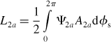
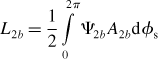
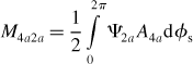
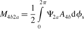
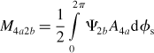
Substituting (6.1–6.4), (6.15–6.18) and (6.6) into the above equations and solving the integrations result in a simple mathematical form. Denoting them in a matrix form
From the above-calculated results, one can see the following:
(a) The self-inductances L4a, L4b, L2a and L2b are a product of airgap permeability, axial length, rotor radius and winding turns, and the inverse of the airgap length.
(b) The mutual inductance M4a4b between the 4-pole windings is zero because windings 4a and 4b are perpendicular to each other. The same is true for M2a2b.
(c) The mutual inductances M4a2a, M4b2a, M4a2b and M4b2b represent the coupling between the 4-pole and 2-pole windings. These mutual inductances are proportional to the rotor radial displacements x and y.
(d) These mutual inductances are zero when the rotor is positioned at the centre. This fact is easily understood because the 4-pole and 2-pole windings are symmetrically wound and are not coupled when the rotor is centred. If these inductances are zero there is no induced voltage in the 2-pole winding when a 4-pole revolving magnetic field is generated. On the other hand, no induced voltage appears at the 4-pole terminals when the 2-pole winding current generates a 2-pole revolving magnetic field. Therefore the voltage requirement for the suspension winding is low.
(e) Radial force is associated with the radial-displacement-dependent inductance terms (6.32) because they represent an imbalance in stored magnetic energy in the airgap. The derivatives (with respect to the radial displacement) of (6.32) are constant, producing constant radial force gains.
Figure 6.10 shows an example of the measured inductances with respect to the radial rotor position. In Figure 6.10(a), the inductances are shown when the rotor is displaced in the x-axis direction; M4a2a and M4b2b are proportional to the rotor displacement x and the mutual inductances M4b2a and M4a2b are almost zero. This corresponds to (6.32). In Figure 6.10(b) it is the mutual inductances M4b2a and M4a2b that are almost proportional to the displacement y. The airgap length of the measured test machine is 0.4 mm. Good linearity is seen up to about half of the airgap length. It is interesting to see this linearity because the equations are derived with an assumption that the rotor radial displacement is small compared to the airgap length.
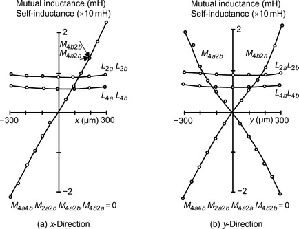
The self-inductances are constant according to (6.30) and (6.31); however, these inductances have a slight minimum value at the centre position. The approximation used to obtain (6.6) neglects the second and higher order terms of radial displacements and there is a small variation with eccentricity in the constant permeance term in (6.6), which is neglected.
Derive the mutual inductance matrix between the 4-pole and 2-pole windings for the alternative winding and coordinate system definitions shown in Example 6.1.
According to the definition in (6.26) M4a2a can be derived for the alternative winding and coordinate system definition as
A similar calculation can be done for the other three elements so that the mutual inductances are derived as
6.6 Radial force and current
In this section the radial forces are derived from partial derivatives of the stored magnetic energy where the stored magnetic energy is calculated from the inductance functions.
In the previous section the inductance functions are derived mathematically. Based on these functions, the relationships between flux linkages and winding currents can be written as
where L4 and L2 are constants, i.e., the self-inductances. M′ is the derivative of mutual inductance with respect to the rotor radial displacement. Let us define a4 × 4 inductance matrix as [L] and define the current vector as [i]. Then the stored magnetic energy Wm is given by
Expansion of the matrix results in
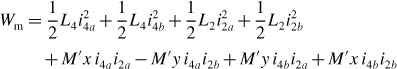
The first four terms represent the stored magnetic energy associated with the self-inductances. The last four terms are the energy terms of the mutual inductances between the 4-pole and 2-pole windings. The radial forces can be derived from the partial derivatives of the stored magnetic energy, assuming a magnetically linear system where
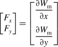
Substituting (6.37) into (6.38) yields a simple mathematical expression because the first line in (6.37) disappears since the first 4 terms are not functions of radial displacement:
The radial forces are expressed as a sum of the current products between the 4-pole and 2-pole windings. The radial forces are proportional to the derivative of mutual inductance M′. This equation can be also written in matrix forms:
In (6.40) the radial forces are expressed as a product of the 2 × 2 matrix of the 4-pole winding currents and the 2-pole winding current vector. This expression is quite useful when i4a and i4b are assigned as the motor currents and i2a and i2b as the suspension winding currents. On the other hand, in (6.41) the 4-pole current vector expresses radial forces so that this equation is useful when the 4-pole winding is assigned as the suspension winding.
Let us assume that the 4-pole winding is assigned as the motor winding so that the 2-phase sinusoidal currents are
and (6.40) is rewritten as
From this equation, the following points can be made:
(a) Relationships between the radial forces and suspension winding currents are modulated by the revolving motor magnetic field.
(b) The radial forces are proportional to the motor excitation current I4.
(c) The radial forces are proportional to the radial force winding currents i2a and i2b.
In comparison to the magnetic bearing, a bias current is not needed in the suspension windings of a bearingless motor. The bias current is replaced by an excitation current I4 in the motor windings. Hence the current requirement in the radial force winding and the driving inverter is proportional to the required radial force. This leads to a lower current requirement in the suspension windings.
In addition, the radial forces are naturally proportional to the suspension winding currents, even without linearization around the operation point (as usually employed in the magnetic bearing using a bias current). It can be said that bearingless motors have inherently linear characteristics due to differential suspension winding operation.
Let us examine a case when sinusoidal currents are used in the 2-pole windings to generate a revolving magnetic field. In this case the 2-pole windings are assigned as the motor windings and the 4-pole windings are used as the suspension windings. For counter-clockwise rotor rotation the currents are
so that (6.41) is written as
From this equation the following points are apparent:
(a) The radial forces are proportional to the 4-pole winding currents i4a and i4b. Hence it is seen that the radial forces are proportional to the radial force currents in both the 4-pole and 2-pole motor cases.
(b) The radial forces are modulated by sinusoidal and co-sinusoidal functions. The frequency of the 2 × 2 matrix is half that in (6.43) because the modulation frequency is determined by the revolving speed of the magnetic field. In (6.45) the magnetic field has one mechanical rotation for one current cycle since the motor windings are 2-pole. However, two current cycles are required for one mechanical rotation when the motor windings are 4-pole, as in the case of (6.43).
Derive the magnetic energy and radial force equations for the alternative winding and coordinate system definitions. Also find expressions for the current for clockwise rotation of the magnetic field.
In the 4 × 4 matrix shown in (6.35), negative signs are seen in elements (1,4) and (4,1). In the alternative definition, these signs are in elements (1,3) and (3,1) only. The stored magnetic energy can be calculated. The result is composed of self-inductance and mutual inductance functions. The self-inductance energy is obtained from the first line in (6.37) and the mutual inductance energy is
so that the radial forces can be written in matrix forms such that
Suppose the 4-pole winding is used as the motor winding. In order to generate a revolving magnetic field in the clockwise direction, the current should be as given in (6.42). Note that a clockwise-revolving magnetic field is generated because the polarity winding 4a is reversed. Hence the radial forces are written as
Note the negative sign in element (1,1).
If the 2-pole winding is used as the motor winding and the revolving magnetic field is in the clockwise direction then
6.7 The dc excitation of the primitive bearingless motor
In this section a dc current is used to excite the motor winding in the primitive bearingless motor. Since dc current generates only a static magnetic field, there is no rotational torque production. Hence it acts as a radial magnetic bearing. A basic controller configuration is introduced. It is shown that the system has good characteristics and can operate as a 3-phase inverter-driven magnetic bearing.
Let us consider that one of the 4-pole winding currents i4a is set to dc current I4, while i4b is zero. This current value provides the condition at ωt = 0 in (6.42) so that the relationships between the radial forces and suspension winding currents are given by (6.43); substituting ωt = 0 gives
This equation can be simplified to
This equation shows the simple relationships between radial force and winding current for a condition shown in the Figures 6.1 and 6.2. Note that the radial force direction in Figure 6.2(a) is negative corresponding to the negative sign in the above equation.
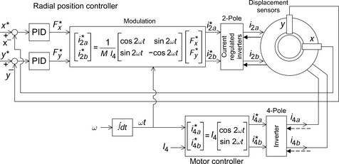
Using the relationships in (6.52) we can design a controller block diagram. In a radial magnetic suspension system the radial force commands of the two perpendicular axes are given by the position controllers, e.g. the PID controllers. Current commands are generated from the controller so that the actual radial forces precisely follow the force commands. Suppose that the radial force commands are generated on the x- and y-axes as F*x and F*y. The current commands i*2a and i*2b should be generated using the above equation so that
The derivative of mutual inductance M′ is a constant determined by the machine dimensions and number of winding turns. The excitation dc current I4 can be kept constant. Thus a simple structure of a radial magnetic suspension system can be designed as illustrated in Figure 6.11.

Figure 6.11 shows a primitive bearingless motor with 4-pole and 2-pole windings. Two shaft displacement sensors are installed to detect the shaft movement in two perpendicular axes. The detected radial positions x and y are compared with these references x* and y*, which are zero in most cases, so that radial position errors are amplified by the radial position controllers as shown by the PID blocks. Radial force commands F*x and F*y are generated, and from these radial force commands the suspension winding current commands i*2a and i*2b are generated by division by the constant M′I4. Note that a minus sign is seen in the y-axis block. The current commands are fed to an inverter to regulate instantaneous current values, which are forced to follow the commands so that radial forces are generated in the bearingless motor. The radial forces therefore track the radial force commands.
In the motor winding, a dc current I4 is supplied to the a-phase winding. The supplied dc current generates a static 4-pole flux distribution. This static field acts as the bias flux as seen in the conventional radial magnetic bearing.
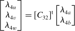
Although 2-phase windings are described for simplicity, 3-phase windings with a 3-phase inverter are usually used so that a 3-phase radial magnetic bearing can be constructed. The 2-phase coordinates can be easily transformed into 3-phase coordinates, as often done in standard electrical motors. This concept is briefly introduced below; however, the details will be shown in the next chapter. The 3-phase and 2-phase current relationships can be related to each other using the matrix
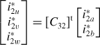
where [C32]t is the connection matrix given by
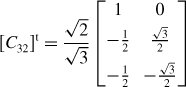
Note that the 3-phase windings have only two degrees of freedom because the sum of the three currents should be zero. Hence the 3-phase currents are directly derived from the 2-phase instantaneous current values. The blocks shown in Figure 6.12 with 3-phase windings can replace the dotted area in Figure 6.11.
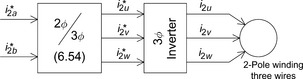
In Figure 6.12 the 2-phase current commands are transformed into 3-phase current commands by equations (6.54) and (6.55). The 3-phase current commands are fed to the 3-phase inverter, which regulates the instantaneous 3-phase currents of the 3-phase suspension windings.
The advantages of having this dc-excited bearingless motor operating as a radial magnetic bearing are summarized as follows:
(a) A low-cost 3-phase inverter power module, including power devices, main circuit connections, gate drive circuits and protection circuits, can be applied to a radial magnetic bearing application.
(b) Only a 3-wire connection is required for 2-axis active positioning.
(c) Software algorithms developed for motor drives can be easily applied.
6.8 AC excitation and revolving magnetic field
In this section, 2-phase ac currents are supplied to the primitive bearingless motor winding set to generate a revolving magnetic field. The rotor is made up of circular laminations of silicon steel so that torque is not generated even though the magnetic field is rotating. Hence this ac-excited bearingless motor is not practical but it does aid analysis and understanding.
Let us suppose that 2-phase currents excite the 4-pole windings as previously shown. Substituting the command values for radial forces and the currents into (6.43) produces current commands. In doing so, it is important to check if the inverse matrix exists for the 2 × 2 square matrix. From a simple calculation it can be seen that the determinant of the matrix is −1. Hence an inverse matrix does exist and it is written as
where φ is equal to 2ωt. This matrix is characterized in such a way that the inverse matrix is exactly the same as the original matrix. This is a kind of unitary matrix. Substituting the commands into (6.43) and solving for the radial force current commands yields
This equation shows how the radial force current commands are calculated from the radial force commands. Figure 6.13 shows the block diagram of the primitive bearingless motor excited with 2-phase ac currents in the 4-pole windings. The radial force commands are fed from the PID controllers to the modulation block, which implements (6.57), so that the suspension winding currents follow the force commands.
The angular speed ω of the current is fed to an integration block with a reset. The integrated output is expressed as ωt. The angular speed can be assumed to be almost a constant in the steady-state conditions and together with the amplitude I4, the 4-pole current commands i*4a and i*4b are generated. These commands are fed to an inverter that regulates the instantaneous currents. The 2-phase ac current produces a 4-pole revolving magnetic field; note that the 2-phase winding case is drawn in the figure for simplicity although a 3-phase winding and 3-phase inverter can be used as shown in the previous section.
If the 2-pole winding is employed as the motor winding then the motor currents are regulated to follow the currents as given in (6.44). In the modulation block, the suspension winding current is obtained from (6.45); substituting the command values for the radial forces and the 4-pole winding current gives
Note that the angular frequency of the motor currents and modulation is ω for the 2-pole motor case and that the negative sign is not in the same position.
Derive the equations for determining the currents of the suspension windings from the radial force commands for both the 4-pole and 2-pole motor cases using the alternative coordinate system definition.
From the Example 6.4, an inverse matrix relationship for the 4-pole motor can be derived, where
6.9 Inductance measurements
In the previous sections, the windings were assumed to be 2-phase. This assumption was made to simplify the analysis. However, in practice, 3-phase windings are usually used because the total number of wires is only 3, compared to 4 for 2-phase windings. Therefore it is quite important to examine the 3-phase winding system. In this section, an example of the 3-phase winding system is introduced. In addition, the inductances of the 3-phase windings are transformed into the 2-phase system and it is shown that considerable simplification is possible by use of 2-phase coordinates.
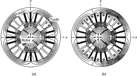
Figure 6.14 shows a cross-sectional view of a stator core with winding conductors. There are 24 slots in the stator. The stator slots contain, alternately, one 4-pole coil-side and one 2-pole coil-side. Coil sides 4u, 4v and 4w are for the 4-pole windings of phase u, v and w respectively. Coil-sides 2u, 2v and 2w are for the 2-pole windings of phase u, v and w, respectively. The coils of 2u are arranged so that a positive current generates an MMF in the x-axis direction only. This arrangement corresponds to winding 2a as shown in Figure 6.6. The coils of 2v and 2w are arranged so that the vector sum of their MMFs is in the y-axis direction when there is positive current in the coils of 2v and an equal but opposite current in the coils of 2w. This arrangement corresponds to winding 2b. The coils of 4u are arranged to correspond to winding 4a and the vector sum of the MMFs due to 4v and 4w align with the 4b winding MMF (again with positive and negative currents in 4v and 4w). The correspondence between the 2-phase and 3-phase windings is important for 3-phase to 2-phase transformation using the matrix in (6.55).
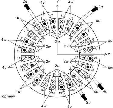
The coil connections are shown for the u-phase windings only. Coil side 4u enters at slot 22 and exits at slot 4. The entry-end is connected to the 4u terminal and the exit-end is connected to the star point 4n. For 2u, the winding enters at slot 20 from terminal 2u, exits from slot 8 and is connected to the 2-pole star point 2n.
Figures 6.15 and 6.16 show the open coil maps. The cylindrical stator core is opened between slots 1 and 24 and linearized. This figure is familiar to coil manufacturers. The first coil of 4u starts from terminal 4u then goes down slot 22 and returns up slot 3. There are several turns of the coil round these two slots before the phase is connected to coils that span slots 21 and 16, 10 and 15 and finally 9 and 4, with the phase winding finishing at slot 4. Coil manufactures wind the copper wires as shown in the figure and then insert coils into stator slots.
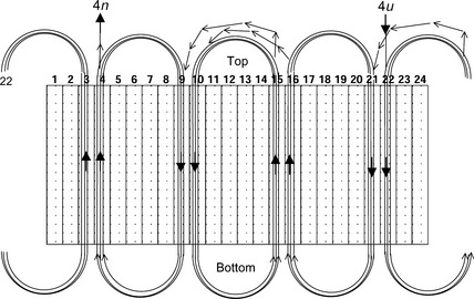
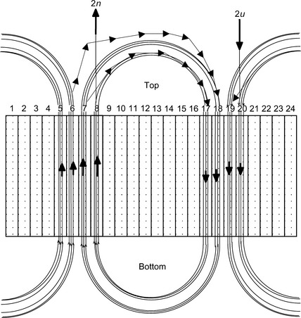
Figure 6.17 illustrates a stator core with both 4-pole and 2-pole windings. The short-pitched (inner) coil ends are for the 4-pole windings, and the long-pitched (outer) windings are for the 2-pole windings. In total there are 6 wires for the winding terminals.
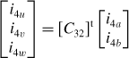
Since there are six terminals for each of the 3-phase windings in the bearingless motor, the relationships between the flux linkages λ4u, λ4v, λ4w, λ2u, λ2v, λ2w and currents i4u, i4v, i4w, i2u, i2v, i2w can be expressed by a 6 × 6 matrix:
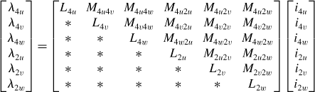
The asterisks* indicate matrix elements that are not written because the matrix is symmetrical. Some of the inductances will be functions of the radial rotor displacement.
Figure 6.18 shows a circuit diagram that can be used to measure the inductances. All the inductances cannot be measured at once. In the figure, 4u is connected to a single-phase ac power supply. The self-inductance L4u is obtained from
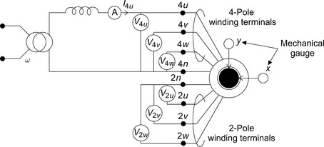
where V4u and I4u are the rms values of voltage and current at terminal 4u, R4u is the winding resistance and ω is the angular frequency of the power source.
The mutual inductances are calculated, for example, from M4u4v = V4v/(ωI4u). The rotor radial positions can be fixed to any desired position within the airgap length between the stator and rotor. The radial displacements are measured by mechanical dial gauges or eddy current position sensors. It is important to move the rotor along one radial axis while keeping the displacement of the other axis zero. Initially the x-axis displacement is zero; V2u can be monitored using an oscilloscope. The induced voltage V2u is proportional to the x-axis displacement so that if the rotor is moved in a positive x-axis radial direction then V2u increases and it is in phase with respect to V4u. If there is a negative displacement along the x-axis, the polarity of V2u is the inverse of V4u. In order to keep the y-axis displacement zero, the difference between V2v and V2w is monitored using an oscilloscope. This voltage difference is proportional only to the y-axis displacement.
Once the radial position is fixed, all the inductances are measured by rotating the winding excitation. First, 4u is excited to measure six inductances, next the winding 4v is excited to measure five inductances and finally 4w is excited to measure four inductances. Then, windings 2u,2v and 2w are excited independently in order to measure all the inductances in the above equation. Once this is done the rotor is moved to the next radial position. When the rotor is displaced, one will see vibration caused by strong radial attractive magnetic force at high current; this vibration should be minimized to reduce measurement errors. However, the current level should be close to the normal motor excitation level to obtain the inductance values at that operating point. To do this, the rotor should be tightly fixed at each measuring point before exciting a winding. One way to fix the rotor is to fabricate a shaft with a large diameter end-disc with a tapped hole, which fixes the rotor shaft to a stationary position with a bolt.
Figure 6.19 shows the inductance variations with respect to a normalized radial displacement xn, which is equal to x divided by the nominal airgap length g0. In the figure, the rotor is displaced by about g0/2. In Figure 6.19(a), the self-inductances and mutual inductances of the 4-pole and 2-pole windings are shown. These inductances are almost constant as expected. If the rotor is moved further, these inductances start to vary as a quadric curve, having the minimum at xn = 0. In Figure 6.19(b), the mutual inductances between the 4-pole and 2-pole windings are shown. Some mutual inductances, for example M4u2v and M4u2w, are the same value because of the symmetrical winding arrangement. In total nine mutual inductances are shown. It can be seen that the slopes of these inductances with respect to the rotor radial displacement are not constant. In a simple theoretical inductance calculation, with a fundamental MMF approximation, only two slopes are obtained; however, the gradient is seen to vary in the figure. This is because of the effects of space harmonics, especially the third harmonic component, in the MMF space distributions. The third harmonic influence is eliminated when transformed into the 2-phase coordinates.
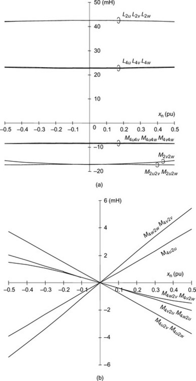
Figure 6.19 3-Phase inductances: (a) self-inductances, mutual inductances between the motor windings and mutual inductances between the suspension windings; (b) mutual inductances between motor and suspension windings
Let us transform these inductance functions into the 2-phase coordinates. Equation (6.61) can be written in a matrix form such that
The 3-phase to 2-phase transform matrix was shown in (6.54) and (6.55). With this transform matrix, the current and flux linkage relationships between the 3-phase and 2-phase representation can be written as

Let us define a 6 × 4 transform matrix as follows:
where [0] indicates a 3 × 2 zero matrix. In 2-phase coordinates the relationship between the flux linkages and currents are expressed by a 4 × 4 inductance matrix as
where


These flux linkage and current vectors correspond to vectors in 3-phase systems and are linked by simple matrices
The original [C6] provides an inverse matrix of the transpose matrix [C6]t. Hence from (6.71), [λ4] = [C6][λ6] and substituting this equation into the left side of (6.67) yields
Substituting (6.62) into the above equation and eliminating [λ6],
Substituting (6.70) an inductance matrix in 2-phase coordinates is derived:
This equation provides the transformation from 3-phase inductances to 2-phase inductances. Therefore (6.74) can be written as
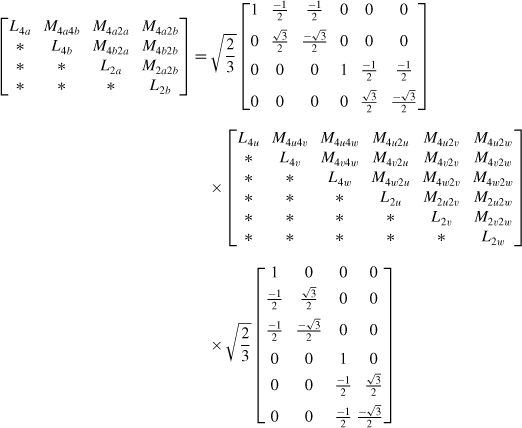
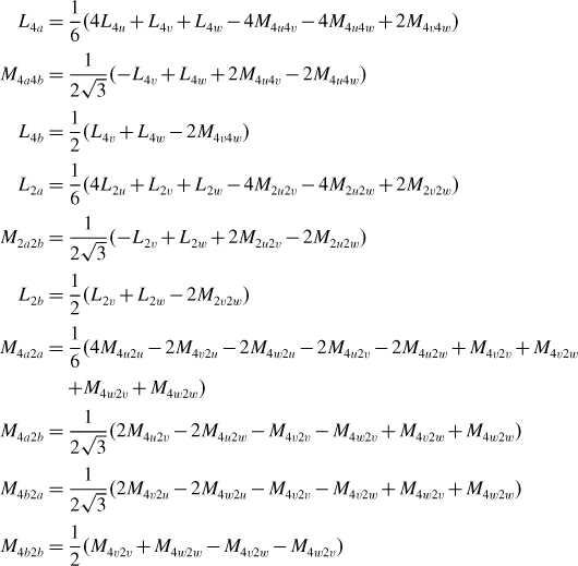
Further calculation of the above matrix equation generates the set of equations below.
The 2-phase inductances above can be calculated by substituting the values shown in Figure 6.19; these are shown in Figure 6.20 for the mutual inductances between the 4-pole and 2-pole windings for both the x and y displacements. In Figure 6.20(a), the inductance values M4a2a, M4b2a, M4a2b and M4b2b are shown, but note that M4a2b and M4b2a are zero while M4a2a and M4b2b are proportional to the radial displacement and have the same slope as M′ = 40 H/m. Quite simple inductance functions are found as a result of the 3-phase to 2-phase transformation. This is the main reason why the analysis was done using 2-phase winding theory in the previous sections of this chapter. In Figure 6.20(b), the mutual inductances are drawn with respect to the y displacement. M4a2a and M4b2b are zero, while M4b2a and M4a2b are almost the same as the absolute value, i.e., a slope of 40 H/m.
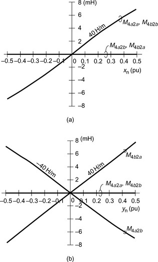
Figure 6.20 Mutual inductance variations in 2-phase coordinates: (a) mutual inductance variation in x-axis; (b) mutual inductance variation in y-axis
The validity of equation (6.35) can be confirmed. Measuring the inductances is the first step in obtaining the machine parameters, and these measurements can be done with simple equipment. The radial force constants can also be obtained, which are necessary to estimate the loop gains of the radial position regulation loops. It is also useful to check to see if windings are correct. If one turn is missing in a certain phase, the inductance values will have slight differences between phases. As shown in (6.30–6.32), the inductance values are proportional to the square of the number of turns so that it is possible to estimate the increase or decrease of inductance when there is one turn too many or too few.