
Magnetic bearing controllers
In the previous chapter, electromagnetic designs and mathematical expressions for magnetic bearings and related actuators were described. The magnetic bearings were modelled as two simple force constants, which were defined with respect to displacement and current. The transfer function is inherently unstable so that the controller design is important.
In this chapter, the basic controller design strategy of a magnetic suspension system is described and discussed in detail. Based on a simple one-axis magnetic suspension system, the design of a proportional-derivative (PD) controller is explained in order to realize simple magnetic suspension. Designs with good frequency and time domain responses are illustrated and disturbance force suppression is also discussed. The one-axis model is extended to a two-axis model. The displacement variations caused by mechanical unbalance and also by eccentric misalignment of a sensor target and a magnetic bearing rotor are included. Finally the application of synchronizing disturbance components is introduced.
3.1 Design principles in one-axis magnetic suspension
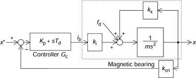
Figure 3.1 shows the block diagram of a magnetic bearing and its controller for one-axis magnetic suspension. The position x of a suspended object is detected and amplified by a displacement sensor with gain ksn and then compared with the position reference x*. The error is amplified by a controller Gc. A current ib is fed to the one-axis magnetic bearing. In the magnetic bearing block, m is the object mass, ki is the force-current factor and kx is the force-displacement factor.
The transfer function of the magnetic bearing is not stable so that the controller must stabilize it using a feedback loop.
A simple controller suitable for a magnetic bearing is a PD controller. The ideal transfer function of a PD controller is
where Kp is the constant gain of the proportional controller and Td is the time constant of the derivative controller. The loop transfer function can be written as
Hence the transfer function from position reference to the displacement is derived to be
Equating the denominator to zero provides a characteristic equation. Solving the equation for s gives
This equation provides some conditions for the magnetic suspension stability:
(a) If Td is zero and Kp = 0 then the value inside the brackets is
Hence one pole is located in the right half plane. This system is unstable.
(b) If Td is zero and Kpkiksn − kx > 0 then
Hence two poles are located on the imaginary axis. Theoretically speaking, this condition is stable; however, in practice, it is not useful since it is marginally stable.
Since two poles are located in the left half plane, the feedback system is stable.
This shows that a derivative controller is necessary to make the magnetic suspension feedback loop stable. In addition, there is a minimum proportional gain for the controller, which is given by Kp > kx/(kiksn). This minimum gain condition is obtained as follows: the radial force is generated by kxx, i.e., a product of a force/displacement constant and displacement. This force makes the magnetic suspension system unstable. Therefore kxx should be cancelled by the negative feedback force in order to make the system stable. The radial force feedback is given by −kiksn(Kp + sTd)x. In steady-state conditions, sTd can be neglected so that the radial force feedback is −Kpkiksnx. Hence the sum of the radial force is kxx − Kpkiksnx. This is negative when Kp > kx/(kiksn) and this condition is necessary for a stable feedback loop.
3.1.1 Equivalent spring–mass–damper system
Figure 3.2 shows a one-axis mechanical system. A mass m [kg] is suspended by a spring and damper. In a steady-state condition, the length of the spring is Xs + x. The spring generates a force ksx, which is proportional to the spring displacement x so that
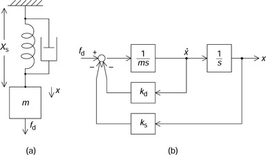
The damper generates a damping force which is proportional to the speed of displacement of x, i.e., kd (dx/dt). An external force fd is also applied to the mass so the motion is governed by the dynamic equation as:
Using this equation, a block diagram can be drawn as shown in Figure 3.2(b). It can be seen that the spring and damper force blocks kd and ks are negative feedback forces. The transfer function is
This transfer function is the typical second-order lag system; the standard form is
where

From these equations the following can be concluded:
(a) The speed of response to the external disturbance force is determined by the natural angular frequency ωn. Faster response is obtained at higher ωn. It can be seen that fast response is realized with a light mass and stiff spring constant.
(b) The damping constant ζ is proportional to the damping constant kd. A strong damper with high kd results in high ζ. For a step input, the response overshoot is not seen if ζ > 1. An estimate gives overshoots of 25 and 50% for ζ = 0.4 and ζ = 0.2 respectively so that an increase in damper constant results in oscillation suppression.
(c) The static displacement is proportional to the spring constant ks. The displacement is small if a stiff spring is employed.
Next, let us look at the similarity between the spring–mass–damper system and magnetic suspension system. Figure 3.3 shows a modified block diagram of the magnetic bearing system previously shown in Figure 3.1. In the figure, a disturbance force fd is applied to the suspended object. Two other forces caused by the object displacement and speed are added. It is assumed that the position reference x* is zero. The similarities between Figures 3.3 and 3.2 can be seen. The constants of the damper and spring are replaced by magnetic suspension system constants such that
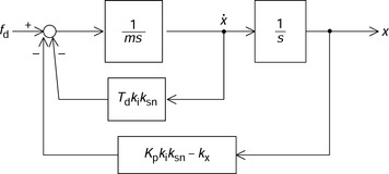
This shows that the time constant Td in the derivative controller is equivalent to the damper constant. In addition, the proportional controller gain Kp is equivalent to the spring stiffness. The damper and spring constants are adjustable in the magnetic suspension system and the force/displacement constant kx results in a negative influence on the spring stiffness. The condition of Kp > kx/(kiksn) produces positive spring stiffness. In practice, kx usually has variations and fluctuations caused by bias current and nonlinearity. Therefore Kpkiksn should be carefully selected to be significantly higher than kx.
From (3.11) to (3.13), the magnetic suspension system is expressed as
where
Hence one can see the following characteristics in the magnetic suspension:
(a) An increase in derivative controller gain results in better damping in response.
(b) An increase in proportional controller gain results in fast response and high stiffness.
Now let us see how we can obtain a stable system with PD controllers. In a practical system, a displacement sensor is used to detect the instantaneous displacement of the suspended object. A displacement of 1 mm gives a 5 V signal, hence the sensor gain ksn is 5000 V/m. Suppose ki = 158 N/A and kx = 1.58N/μm in the radial magnetic bearing example in the previous chapter. Also suppose that m = 3.14 kg and includes the shaft mass. These values are used throughout this chapter unless otherwise specified. Obtain the following:
(a) Draw the bode plot of Gp, i.e., a transfer function of sensor output by input current.
(b) Draw the bode plot for a PD controller with Gc = 10(0.001s + 1).
(c) Find the loop gain. Also draw the bode plot. Specify the phase margin.
(a) The Gp transfer function is Gp = ksnki/(ms2 − kx). Substituting the values yields
The bode plots are drawn in Figure 3.4(a). At low frequency the gain is (kiksn/kx) = −6 dB with a phase delay of 180 deg. At an angular frequency of ![]() , the gain decreases at a rate of −40 dB/dec.
, the gain decreases at a rate of −40 dB/dec.
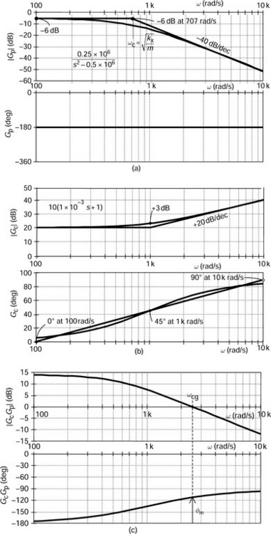
Figure 3.4 Controller design principle in frequency domain: (a) magnetic bearing Gp; (b) controller Gc; (c) loop transfer function GpGc
(b) Figure 3.4(b) shows the bode plots for the transfer function Gc of the PD controller. At low frequency, the gain is 20 dB with a phase lead of 0 deg. In the line approximation, the gain increases at a rate of 20 dB/dec. The numerically calculated characteristics are 3 dB higher than the approximated line at the crossover angular frequency of 1 krad/s. A line approximation is also drawn in the phase characteristics. The line links the three points. One is 45 deg at 1 krad/s. The other two points are 0 and 90 deg at 100 rad/s and 10 krad/s. The numerical calculation shows a good correspondence of the simple line approximation. The important characteristic is that a phase lead is provided in the PD controller. This phase lead gives a phase margin to make the system stable as shown in the next bode plots.
(c) The loop transfer function GL is the product of Gc and Gp (plant and controller transfer functions). The product becomes a sum of the gains when the gain characteristic is on a logarithmic scale. At low frequency the gain is 20 − 6dB = 14 dB. At 707 rad/s, the plant gain decreases at 40 dB/dec, although the controller gain increases at 20 dB/dec from 1 krad/s so that the loop gain decreases at 40 dB/dec and then at 20 dB/dec. As a result of numerical calculation, the loop gain is 0 dB at a gain crossover angular frequency ωcg of 2300 rad/s.
At this angular frequency, the phase angle is slightly advanced from −180 deg due to the phase-lead angle of the PD controller.
The advanced angle generates the phase margin φm and this margin must be positive for stable suspension. If a loop transfer function can be approximated as a second-order lag system, the relationship between the damping constant and phase margin is well known. The damping constant ζ is approximately 0.2, 0.4 and 1 at φm angles of 25, 45 and 75 deg respectively so that larger φm results in better damping of the response.
(d) Figure 3.5 shows the calculated response of the sensor output xsn with a unit step input in x*. A 7% overshoot results at 1.8 ms. It is quite important to see the correspondence between the loop transfer function and this step response. The response time can be roughly estimated from the loop transfer characteristics. The gain-crossover angular frequency ωcg is about 2.3 krad/s in Figure 3.4(c) so that π/(2.3 × 103) = 1.4ms. In this case, the estimated time of 1.4 ms is close to 1.8 ms. It is usual to find that π/ωcg provides an estimated time when overshoot occurs. Strictly speaking, the denominator should be corrected for a damping constant and the second-order lag approximation should be applicable.
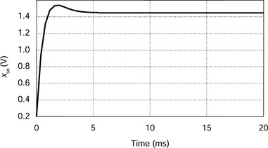
As for the overshoot, a rough estimation is also possible from loop frequency response. The phase margin is about 70 deg in Figure 3.4(c). This value is slightly smaller than 75 deg, which corresponds to ζ = 1 when no overshoot exits. A phase margin of 45 deg corresponds to ζ = 0.4 with an overshoot of 25%. About 10% overshoot is reasonable.
3.2 Adjustment of PID gains
In this section, gain optimization in the PD controller is discussed and practical derivative and integral controllers are introduced. The disturbance force suppression characteristics are examined with adjustment of the proportional-integral-derivative (PID) controller gains.
In a magnetic suspension system, the displacement reference is usually set to zero at the nominal position. For example, the position reference is always the centre position in a magnetic bearing system. The displacement response with respect to the reference is not usually discussed; rather it is the displacement response to a disturbance force that is addressed, although improvements in the disturbance force suppression also result in a better response to the displacement reference. Therefore the displacement response with respect to the disturbance force is examined in this section.
From Figure 3.3, the transfer function from the disturbance force to the displacement, i.e., the dynamic stiffness, is
Note that the denominator is the same as the transfer function of x/x*, as shown in (3.3). Therefore these transfer functions have the same pole loci. This fact indicates that a better response can be obtained in x/x* if the response of x/fd is improved, illustrating the statement made above. In steady-state conditions the static stiffness is obtained by substituting s = 0 so that
This static stiffness provides information about the static displacement from the nominal position. Let us examine the static stiffness. When a mass of m is levitated by the electromagnet, the displacement is Xs. When an additional mass of m′ is added the displacement increases to Xs + x. An increase of x results from the additional external force of m′ga. Based on (3.21), Xs = mga/(Kpkiksn − kx) and Xs + x = (m + m′)ga/(Kpkiksn − kx). If (Kpkiksn − kx) is high, a small displacement and hence high stiffness are obtained.
Suppose that a step disturbance force of 1 N is applied to the suspended object given by the parameters in the previous example. Construct a block diagram for digital simulation. Find the responses at half and twice of the proportional gain. Also find the responses at half and twice the derivative gain. Show the bode plots for these cases. Sweep the disturbance frequency and observe the response.
Figure 3.6 shows a block diagram for digital simulation. A step disturbance is applied to the magnetic bearing. The displacement is amplified by a negative sensor gain for negative feedback. Kp and Td are the proportional and derivative gains respectively. In the digital simulation, a transfer function of (0.01s + 1) is multiplied by the first-order lag element of (10−6s + 1)−1 with a high cut-off frequency of 106 rad/s. This lag element is necessary even in digital simulation. The lower cut-off frequency is usual for practical implementation. The outputs of these controllers are added and it is assumed that the amplitude of the current driver is unity. Therefore the output of ki is a negative feedback force.
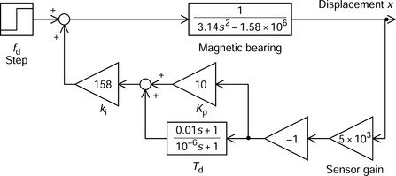
Figure 3.7(a) shows the displacement responses for the given proportional gains. It is seen that the steady-state displacement is smaller for a high proportional gain. The final values are small for high Kp because the static stiffness is high. Figure 3.7(b) shows the displacement responses for the given derivative gains. Improved damping is seen for high Td but the final values are not dependent on Td.
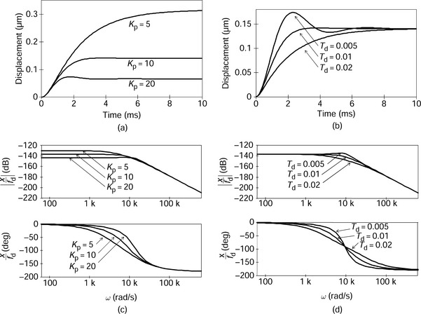
Figure 3.7 Displacement response with respect to disturbance force: (a) displacement time response and Kp; (b) displacement time response and Td; (c) displacement frequency response and Kp; (d) displacement frequency response and Td
Figure 3.7(c,d) shows the bode plots for the dynamic stiffness x/fd. The gain is about −140 dB at low frequency. This gain corresponds to a static stiffness of 0.158 μm/N since 20 log10(0.158 × 10⁻⁶) = −136dB. A discrepancy of stiffness for proportional gains is seen only at low frequency. The magnitude of x/fd is low for high Kp, resulting in better disturbance force suppression. At high frequency, the stiffness does not depend on the PD controller gains. This is represented by a line which decreases with frequency. In this region, the mechanical inertia prevents vibration.
The phase angle of x/fd is also important in testing the magnetic suspension system. In frequency response measurement, an electrical disturbance signal is injected into the magnetic suspension system. The frequency of the injected signal is varied from low frequency to high frequency to observe a wide frequency transfer function. In such a test, the phase angle of the displacement response is in phase at low frequency; however, the phase angle is gradually delayed with increasing frequency. This phase delay is shown in the figure as the phase angle.
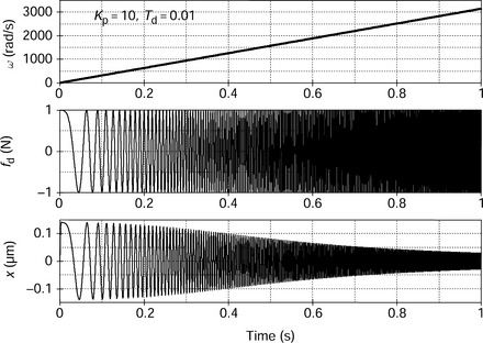
Figure 3.8 shows the disturbance frequency, disturbance force and displacement. The frequency of the disturbance force is increased linearly while the amplitude is kept a constant value of 1 N. As the frequency increases, the displacement decreases as expected from the bode plot. The phase angle is difficult to see from Figure 3.8; however, the displacement phase angle is gradually delayed with respect to fd as the frequency increases.
3.2.1 PD gain adjustment
Better dynamic response of the disturbance force suppression can be obtained in a system with improved damping with fast response. Adjusting the derivative and proportional gains individually does not lead to the required response in a straightforward manner. It is important to increase both the derivative and proportional gains whilst maintaining a certain relationship. This is based on equations for the proportional and derivative gains that are given for a required natural frequency and damping factor. In the previous section, the natural angular frequency and the damping factor are expressed in (3.17) and (3.18) as

From these equations, the proportional and derivative gains can be expressed as
The following observation can be made from these equations:
(a) For a fast response, the natural angular frequency ωn should be high. To increase ωn, the proportional gain should be increased as the square of ωn.
(b) The derivative gain should be increased in proportion to ωn and ζ.
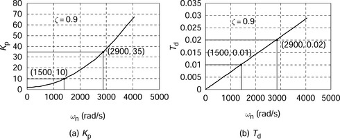
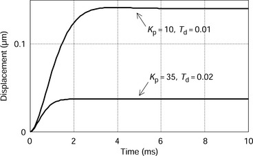
Find the proportional and derivative gains as a function of the natural angular frequency for a damping factor of 0.9. For the cases of Td = 0.01 and 0.02, find the corresponding proportional gain and natural angular frequency. Show the response of the displacement for a step disturbance force of 1 N.
From (3.24) and (3.25), Kp and Td are calculated as shown in Figure 3.9(a,b). From this figure, it can be seen that the natural frequencies ωn = 1500 and 2900 correspond to Td = 0.01 and 0.02 respectively. The corresponding proportional gains are 10 and 35. For a step disturbance, the displacement responses are shown in Figure 3.10. High controller gains result in a fast response with small displacement.
3.2.2 Practical derivative controller
The transfer function of a derivative controller is proportional to s in the Laplace domain. In the frequency domain, this is replaced by jω, so that the magnitude is proportional to the frequency. In practice, the output of an ideal derivative element unfortunately includes considerable noise. High-frequency noise at the input terminals results in significant amplification at the output terminals so that the ideal derivative should be avoided in practice.
Figure 3.11 shows ideal and practical derivative controllers. In the practical controller, the transfer function is known as a phase-lead compensator. This transfer function acts as a derivative function in the angular frequency range of 1/Td ![]() ω. The denominator determines the high frequency limit, which is ω = 1/Tf. Thus, the practical derivative block executes a derivative function in the range 1/Td
ω. The denominator determines the high frequency limit, which is ω = 1/Tf. Thus, the practical derivative block executes a derivative function in the range 1/Td ![]() ω
ω ![]() 1/Tf. The low frequency gain is 0dB and the high frequency gain is limited to Td/Tf. Therefore the engineer can determine Td/Tf from the signal conditions. Note that, in practice, additional high-cut filters are usually employed above 1/Tf to aid rapid cut-off. The proportional term in the numerator can also be eliminated when a proportional controller is connected in parallel.
1/Tf. The low frequency gain is 0dB and the high frequency gain is limited to Td/Tf. Therefore the engineer can determine Td/Tf from the signal conditions. Note that, in practice, additional high-cut filters are usually employed above 1/Tf to aid rapid cut-off. The proportional term in the numerator can also be eliminated when a proportional controller is connected in parallel.
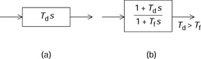
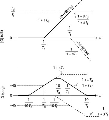
Figure 3.12 shows the bode plots drawn with line approximation. The magnitude is 0 dB at low frequency; however, it increases at ω = 1/Td by 20 dB/dec up to ω = 1/Tf where the magnitude levels out to a constant of Td/Tf. For the phase angle, phase advancement starts at ω = 1/(10Td), with 45 deg lead at ω = 1/Td. If 1/(10Tf) is low compared with 10/Td, as found in practice, the phase lead is flat in the frequency range of 1/(10Tf) to 10/Td, then it begins to decrease. The phase-lead angle is 45 deg at ω = 1/Tf, then becomes zero at ω = 10/Tf.
(a) Draw the bode plots for a practical derivative controller Kp + (1 + sTd)/(1 + sTf) for the cases of Td = 0.01 and Tf = 10−6, 10−4 and 10−3.
(b) Apply the above controls to the previous example of the one-axis magnetic suspension. Draw the bode plots and show the phase margins.
(c) Show the displacement response for a step disturbance force. Discuss the Tf selection.
(a) Figure 3.13(a) shows the magnitude and phase characteristics for the given Tf. The case of Tf = 10−6 is close to the ideal case for the drawn frequency range. The magnitude increases at a rate of 20 dB/dec at an angular frequency of 1 krad/s. At this angular frequency, the derivative block gain is equal to the proportional gain so that the phase-lead angle is about 45 deg. The phase-lead angle is close to 90 deg at high frequency. For the case of Tf = 10−4, the magnitude is 20 dB/dec for 1 dec from 1 to 10krad/s. The high frequency limit of 10krad/s corresponds to 1/Tf. The phase-lead angle decreases when the frequency is more than 1 krad/s. For the case of Tf = 10−3, the phase-lead angle is only 20 deg.
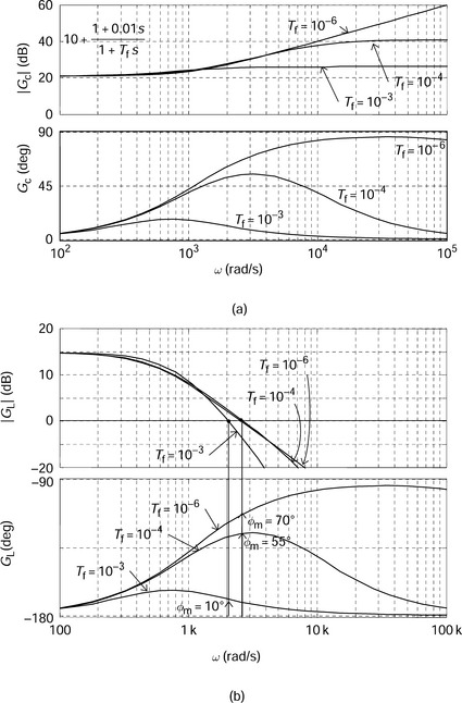
Figure 3.13 Practical PD controller and loop transfer function variations with Tf: (a) practical derivative controller; (b) loop transfer function variation with Tf
(b) Figure 3.13(b) shows the bode plot of the loop transfer function. It is seen that, for the cases of Tf = 10−4 and 10−6, the characteristics are similar, although there is a slight decrease in phase margin. However, for the case of Tf = 10−3, the phase margin is only 10 deg, which is a significant decrease when compared to the cases of 55 and 70 deg for Tf = 10−4 and 10−6. A phase margin of 10 deg indicates insufficient damping. If we draw the x/fd bode plot, Tf = 10−3 has a peak, which indicates vibration at a peak frequency of 2000 rad/s (318 Hz).
(c) The figure is not shown for the displacement time responses for a step disturbance force applied to the suspended object. However, for the case of Tf = 10−3, poorly damped vibration would be seen. The vibration term is about 3 ms, which corresponds to 318 Hz. For the other two cases, well-damped responses would be seen. One can conclude that Tf = 10−4 is the best choice from these three cases, because the noise is less than for the Tf = 10−6 case, while a similar response is obtained.
3.2.3 Steady-state position error and integrator
With only a PD controller, the airgap length between the suspended object and the electromagnetic actuator is increased when external static force is applied due to the steady-state error. In many applications, an integral controller is often employed in addition to a PD controller to prevent this.
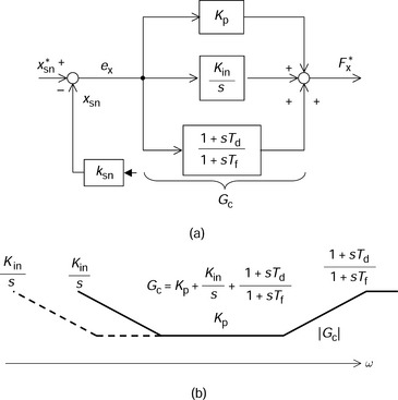
Figure 3.14(a) shows the block diagram for a PID controller. In addition to a PD controller, an integrator Kin/s is added. The input, i.e., a position error ex, is integrated and the output is added to that of the PD controller so that the force command F*x is generated.
The function of the integrator can be explained by Figure 3.15. This figure shows output waveforms with a step input in position reference. At 5 ms, a transient response of the PD controller has almost finished. xsn has overshoot with respect to reference xsn* so that the position error is negative. However the output of the integrator is negative and levels out with time. But an x-axis force is generated in the negative direction. The force tries to move the object in the opposite direction to the x-axis so that the position xsn gradually decreases. The integrator output decreases until the position is on the reference. At a time of 30 ms xsn* is equal to xsn and the integrator output is constant (which is called the integrator constant). Hence F*x is not zero, but is a constant value, which is necessary for force equilibrium for zero position error.
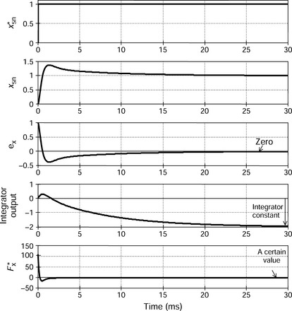
Figure 3.14(b) shows a simplified bode plot for the PID controller. In the mid-frequency range the proportional gain is dominant; however, at low and high frequency ranges, the integral and derivative controllers play important roles. The dotted line indicates a case with low integral controller gain. It can be seen that the magnitude of controller gain Gc is increased at low frequency ranges, thanks to the integral controller. This fact indicates that the loop gain is increased at low frequency so that the negative feedback is improved.
Let us examine the displacement error in the steady-state condition. The displacement error/position command and the displacement/disturbance force can be written as a function of the controller gain Gc, where
Let us substitute for Gc using the following equation:
Further, calculation of (3.26) and (3.27) can be executed. The results are not shown here; however, the results have the operator s in the numerator so that there is a zero at the origin. For a step response the final values are
These values are zero. Hence the steady-state position error is eliminated.
Draw the bode plot for a PID controller with the cases of Kin = 0, 100, 1000 and 10 000 and the parameters Kp = 10, Td = 0.01 and Tf = 10−4. Also draw the bode plot of the loop transfer function and dynamic stiffness with ksn = 5 × 10³ and ki = 158 N/A. Show the step response of the disturbance force suppression.
Figure 3.16(a) shows the bode plots of the PID controller. The low frequency characteristics depend on the integrator gain Kin. When Kin is zero, i.e., equivalent to the PD controller, the magnitude is a constant value, i.e., about 20 dB, which is mostly determined by the proportional controller gain of 10. However, the magnitude increases as the frequency decreases with other Kin values. When Kin = 100 the magnitude increases at an angular frequency of less than 10 rad/s. The flat magnitude frequency range is 10 to 1 krad/s. In the case of Kin = 1000, it increases when the frequency is less than 100 rad/s. It can be said that the latter case is more effective for low frequency disturbance suppression. In the case of Kin = 10000, one cannot observe the flat frequency response. This condition results in a decrease in phase-lead angle at a frequency of around 1 krad/s.
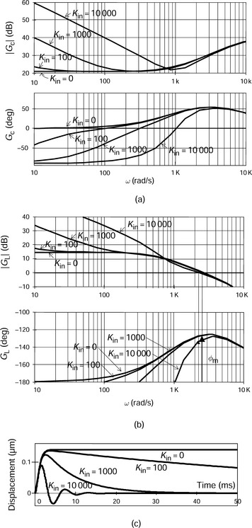
Figure 3.16 Effect of an integrator: (a) frequency characteristics of a PID controller; (b) loop transfer function with several integrator gains; (c) displacement response
Figure 3.16(b) shows the bode plots of the loop transfer function. One can see that high loop gain is obtained with high Kin at low frequency. In addition, a decrease in phase margin is seen for the case of Kin = 10000. Therefore among these four cases, Kin = 1000 is the best choice due to the following reasons: (a) high loop gain in the low frequency range and (b) no decrease in phase margin.
Figure 3.16(c) shows the displacement response with a step disturbance force. For the case of Kin = 10000, poor damping can be seen. When Kin = 100, the displacement response is slow. When Kin = 0, the displacement does not converge to zero. Therefore the best response is obtained at Kin = 1000.
The bode plots for x/fd are not shown here; however, one would see that x/fd is lower, i.e., high stiffness is obtained, for high Kin. For the case of Kin = 10 000, a peak would be observed at 1 krad/s. It can be seen that a peak in stiffness should be avoided to enable damped responses.
3.2.4 Influence of delay
In an actual magnetic suspension system there are many causes of possible delay. The delay may be due to the following reasons:
(a) Iron losses in the actuator iron core.
(b) Flux delay with respect to current, caused by eddy current.
(c) Voltage saturation in a current driver.
(d) Limited frequency response of a current driver.
(e) Limited sensor frequency response.
(f) The sampling period of a digital controller.
(g) An analogue or digital filter at an A/D converter input.
(h) The first-order lag element of a winding resistance and an inductance.
Depending on the application, some of these points may cause serious problems. Therefore it is important to see the influence of delay in a magnetic suspension system. In this section, an example is given to show how the delay could ruin the stability in a magnetic suspension system.
Let us suppose that a first-order lag element, representing the delay, exists in a magnetic suspension system. Let us assume that the cut-off frequency of the lag element is 500 Hz so that a transfer function of [1 + s/(2π500)]−1 is connected in series with the magnetic bearing. Compare the frequency responses of the loop transfer function and dynamic stiffness with and without the lag element. Consider the loop gain adjustment and show the displacement variation when a 100 N radial force is applied with a frequency range between 0 and 500 Hz. Also compare the step disturbance force suppression.
Figure 3.17(a) shows a block diagram for digital simulation. The first-order lag element is connected just after the magnetic bearing block. The PID controller gains are adjusted using the parameters quoted.

Figure 3.17 Simulation blocks and influence of phase lag element: (a) one-axis magnetic suspension system with a delay element; (b)loop transfer function and phase margin
Figure 3.17(b) shows the bode plots of the loop transfer functions with and without the phase-lag elements. It can be seen that there is significant discrepancy in the phase angle characteristics. The phase margin decreases from 50 to 20 deg. In addition, the phase angle is less than −180deg at high frequency. This fact suggests that this is one of the important practical aspects in loop gain adjustment. If the loop gain is increased, for example, by 10 dB, then the gain crossover frequency is 4.2krad/s, where the phase angle is less than −180 deg. Therefore the magnetic suspension loop would not be stable. On the other hand, if loop gain is decreased by 12 dB, then the gain crossover frequency is 400 rad/s, where the phase angle is again less than −180 deg. Hence, in this example, the magnetic suspension is stable only when the loop gain variation is within the range from −12 to +10 dB if there is a lag. In practice, it is usually found that the gain adjustment is difficult to set until a stable point is obtained. If the integrator is eliminated, the low frequency restriction disappears and low loop gain is acceptable. Therefore adjusting the controller gains becomes easier.
If the dynamic stiffness x/fd characteristic is drawn then there is a peak in the magnitude at an angular frequency of 2200 rad/s with a phase lag (which corresponds to 350 Hz).
Waveforms with a sinusoidal sweep in disturbance force input can also be drawn. If the disturbance force has an amplitude of 100 N with a frequency range from 1 to 500 Hz linearly, the displacement x is about 15 μm at low frequency. However, a peak exists at 350 Hz, after which the displacement decreases significantly. These characteristics correspond to the magnitude and frequency characteristics of the dynamic stiffness. The current also has a sinusoidal waveform with peak amplitude at 350 Hz.
A displacement response characteristic can also be drawn when a step disturbance force of 100 N is applied to the suspended object (though not drawn here). It would be seen that the damping is inferior in response when the phase-lag element is included. In addition, a significant fluctuation in feedback force fNFBx would be observed.
In this example, it is shown that the first-order lag element causes a serious problem. In this case the cut-off frequency is 500 Hz; however, it is obvious that the lower cut-off frequency results in instability. For practical implementation, attention should be paid to the elimination of slow response due to the influences listed in (a–h) earlier.
3.3 Interference in two perpendicular axes
The generated radial forces are aligned on two perpendicular axes which usually coincide with the x- and y-axis displacements. However, there are some causes of radial force misalignment, i.e., when they may not be aligned with the x- and y-axes. Suppose that an electromagnet of a radial magnetic bearing is constructed with a misalignment at an angle with respect to the radial displacement sensors. The direction of the generated radial force has an angular position error, which results in interference of x- and y-axis force components. There are several other possible causes of interference, as listed below:
1. Flux due to eddy currents can generate a delay in the radial force. At high rotational speed and with a solid rotor, eddy currents flow on a rotor surface, which generates phase-delayed components in the flux wave distribution with respect to the rotor. This phase lag in the flux results in a direction error for the generated radial force.
2. The gyroscopic effect is apparent with short-axial-length machines with large-radius rotors. The gyroscopic effect generates interference radial force.
3. In bearingless motors, the radial force direction includes errors if the controller has errors in the estimated or detected angular positioning of the revolving magnetic field. Also direction errors can be caused by space harmonics of MMF and permeance distribution.
The interference between the x- and y-axis radial forces can cause a serious problem. In this section radial interference and its influence in the feedback system are examined.
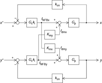
Figure 3.18 shows two perpendicular axes x and y as well as the feedback radial forces fNFBx and fNFBy with slightly delayed angular position. The rotor is rotating in a counter-clockwise direction. The direction angle error is defined as θer and the interference radial forces can be written as:
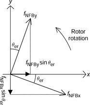
Figure 3.19 shows a block diagram that includes the interference. The outputs are the radial positions and the inputs are the references. The upper and lower blocks are for x- and y-axis dynamic models. The interference is generated by Kmx and Kmy. The decrease in radial force due to cos(θer) is neglected because θer is small.
Let us apply a step reference in x* and see the response of displacement x. Figure 3.20(a) shows the step responses. The parameter Km is set as Kmx = −Km and Kmy = Km. A serious damping problem is seen when Km is increased. If Km is increased to more than 0.3, which corresponds to a 17 deg direction error, the negative feedback has difficulty in damping the system.
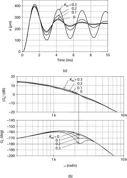
Figure 3.20 Step response and frequency characteristics: (a) displacement response with interference gain variations; (b) loop transfer function and phase margin
Figure 3.20(b) shows the loop transfer function of the x-axis system. At an angular frequency of 2200 rad/s, a large phase delay is seen which increases with Km. In an acceleration test, with Km = 0.3, high vibrations are observed, again, at a speed of around 2200 rad/s. Also the dynamic stiffness is low around this angular frequency.
To see the results of digital simulation, it is also important to analyse the influence of the interference. In Figure 3.19, the radial position reference x* is compared with radial displacement x, then amplified by PID controller gain Gc and ki. A disturbance force fdmx is added and the sum of radial force is applied to the magnetic bearing system Gp, so that the radial displacement x is given. The same structure exists for the y-axis.
Suppose that the y-axis position command y* is zero; in practice, this assumption is valid in most cases so that the block diagram of the interference from fNFBx to fdmx is simplified as shown in Figure 3.21. It can be seen that the interference is represented by two series blocks that have inputs fNFBx and fdmx. The block transfer function is
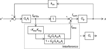
It is important to examine the transfer function of fdmx/fNFBx. Let us define Gi = fdmx/fNFBx. Gi is the transfer function of interference. If Km = 0 and Kmx = Kmy = 0 then Gi = 0, hence there is no interference. The fraction part is quite interesting: GpGcksnki is the loop transfer function of the radial magnetic bearing without interference so that GpGcksnki is high at low frequency. However, it decreases at a frequency determined by the mass and spring constants as previously shown in section 3.1. The fraction part transfer function is near unity at low frequency.
Figure 3.22(a) shows the transfer function of Gi for Km = 0.1 to 0.3. It can be seen that the low frequency gain is proportional to K2m. At 2200 rad/s the magnitude of Gi exhibits a peak, then it decreases in the high frequency range.
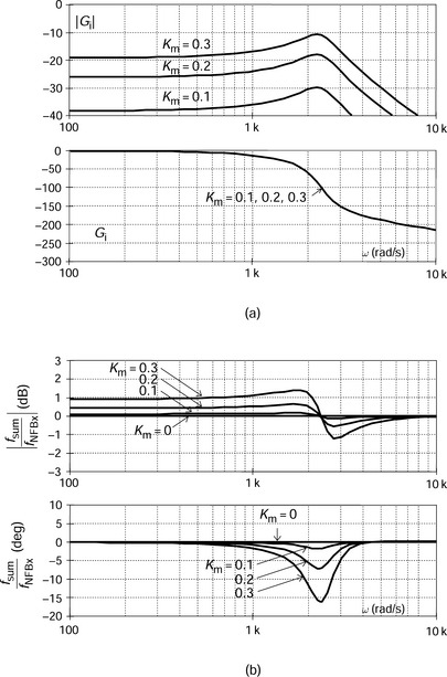
Figure 3.22 Interference frequency characteristics: (a) interference transfer function Gi; (b) bode diagrams of interference
The interference force fdmx is added to the normal feedback force fNFBx in parallel. Therefore the transfer function from fNFBx to the sum of radial force fsum is written as
Figure 3.22(b) shows a transfer function of fsum/fNFBx. The magnitude is close to 0 dB. The important point is that there is a phase lag at around 2200 rad/s. The phase lag characteristic of fsum/fNFBx is not a common shape. This is explained by (3.34). The 1st proportional term is dominant across most of the frequency range so that the phase angle is 0deg both in the low frequency and high frequency ranges. However, the second term has influence at a certain frequency, i.e., 2200 rad/s in this case, because it has a peak. At around the peak frequency, the phase angle rotates significantly. Hence the phase angle of fsum/fNFBx is delayed only at 2200 rad/s. This angular frequency is always close to the gain-crossover angular frequency because the fraction part in the second term is the closed-loop gain of the magnetic bearing. Therefore the interference can be a serious problem in a two-axis magnetic suspension system. Solutions are dependent on the causes of the interference. Steps should be taken to try to eliminate the misalignment of radial forces and x- and y-axis coordinates when designing a system.
3.4 Unbalance force and elimination
Vibration is caused by mechanical unbalance in a rotating system. In this section, the principles and mathematical representation of unbalanced mechanical force are introduced and the influence on the magnetic bearings is shown. An elimination method for unbalanced disturbance is included.
Figure 3.23 shows the principle of unbalance force generation. The x- and y-axes are perpendicular axes in a stationary frame. The shaft is perfectly symmetrical but there is an additional mass of me at a radius of ε in the direction of ωrm t, where ωrm is the rotational angular speed of the shaft. The radial forces in the two perpendicular axes are defined by
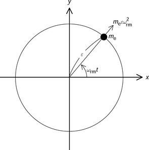
These radial forces are synchronized to the shaft rotation. The amplitude is proportional to the square of rotational speed. The synchronous vibration is caused by an unbalanced force in the two-axis magnetic bearing.
Figure 3.24 shows a simplified block diagram. The signal generator generates unbalanced radial forces for the case of meε = 10−6. These forces are added, as disturbance forces, to the negative feedback forces fNFBx and fNFBy. A similar system exists for the y-axis.
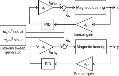
Figure 3.25(a) shows the waveforms for a rotational angular speed ωrm, disturbance forces fdx and radial position displacement x. The rotational speed increases as a ramp function. At a time of 1 s, the rotational speed is 6282rad/s, i.e., 1000 r/s or 60 000r/min. The following facts are obvious:
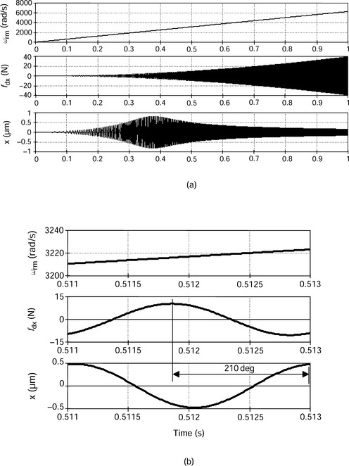
(a) At low rotational speed, the radial displacement increases with speed because the unbalanced force increases with speed.
(b) At a time of 0.37 s, the displacement is at the maximum value. This maximum vibration occurs at a rotational speed of about 2300rad/s. This is the critical speed.
(c) At high rotational speed, the displacement decreases even though the amplitudes of the unbalanced forces are increasing. This decrease is caused by the shaft mass.
Figure 3.25(b) shows enlarged waveforms at around the 0.51 s point. The displacement is delayed by about 210 deg with respect to the disturbance force at a speed of 3200rad/s. It can be seen that the delayed angle of the displacement is speed dependent and this is for the reasons described below.
If a bode plot is drawn for the transfer function from the disturbance force to the displacement x/fdx then the following correspondence can be seen between the bode plots and time domain responses:
(a) The magnitude of x/fdx is high in the speed range of 100–2000 rad/s, with a peak at about 2000 rad/s.
(b) The phase angle of x/fdx has strong frequency dependence. At low speed, the phase angle leads; however, there is a gradual phase decrease as the speed increases. At 500 and 3250 rad/s, the phase delay angles are 18 and 214 deg respectively. These phase delay angles correspond to the time domain waveforms in the enlarged waveforms.
3.4.1 Synchronous disturbance elimination
As a result of the unbalance force, radial vibrations occur; these are synchronized to the shaft rotation so that the frequency of the vibrations increases with speed. Current drivers have to provide high frequency currents to magnetic bearings. The impedance of the magnetic bearing winding is approximated to ωL, where L is the inductance. The back electromotive force (EMF) is proportional to the rotational speed so that the voltage requirement increases. If the current driver cannot deliver enough voltage to provide current to the windings, the current driver becomes saturated so that the negative feedback is opened. Since the magnetic suspension system is unstable without the feedback, the system becomes unstable, which may result in shaft touch-down to the emergency bearings. Therefore it is important to eliminate the synchronous disturbance components from the negative feedback loops. In this section, a method of eliminating the synchronous disturbance is introduced. This method reduces shaft vibrations and the synchronized components in the current drivers.
The principles of synchronized disturbance elimination are explained below.
(a) Detect only the synchronized components from the detected radial positions.
(b) Subtract the detected components from the radial positions. Therefore only the synchronized components are eliminated from the radial positioning.
In power electronic applications, synchronizing a disturbance to eliminate it – i.e., stabilizing the voltage on a commercial power line – is often done by the controller. The same concept can be applied here.
A coordinate transformation from stationary x- and y-axes to rotational Xd- and Yd-axes is given by
where ωrm t is the detected shaft rotational position. If radial displacements x and y include the synchronized components then Xd and Yd include dc components. Low pass filters can be used to detect only the dc components of Xd and Yd. Let us define the dc components as X′d and Y′d. Therefore, the coordinate transformation from rotational axes to stationary axes of these dc components is
where Xsync and Ysync are the synchronized components of x and y.
Figure 3.26 shows a block diagram of a synchronizing component eliminator. From x and y, the equations (3.37) and (3.38) are calculated, hence Xsync and Ysync are obtained. These are the detected synchronized components of x and y. These are subtracted from x and y so that xcom and ycom are obtained. These displacements do not include the synchronized components with angular frequency of ωrm.
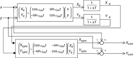
Figure 3.27 shows the effects of synchronized disturbance elimination. The shaft is rotating at a constant speed of 30 000 r/min. The synchronized disturbance elimination is switched on at a time of 0.4 sec. The disturbance force caused by unbalance is fdx. Before the elimination function is switched on, the radial displacement x and feedback radial force fNFBx are fluctuating. Once it is switched on the feedback radial force fNFBx is significantly reduced. Since the winding current is proportional to the feedback radial force, the winding current is also decreased. In addition, the vibration of the radial displacement x is reduced.
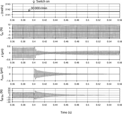
Let us look at this in the detail. Before switch-on, the synchronized component Xsync is detected so that xcom is almost zero. After switch-on, a transient condition is started, lasting about 0.1 s, for which the time constant is mainly determined by the low pass filter. In this simulation, the cut-off frequency is set to 2 Hz. Once Xd approaches the final value, Xsync has constant amplitude, while xcom is almost zero.
Is the system stable if the synchronized components are eliminated from the negative feedback loops? The synchronized disturbance elimination is effective only when well over the critical speed. The eliminator is not effective, and is rather problematic, at low rotational speed and when the magnetic bearings need damping because the operation happens to be either under or slightly over the critical speed.
There are several other methods to reduce the current and displacement caused by the unbalance force. The disturbance forces are given in (3.35) and (3.36), and if identical electromagnetic forces are generated in the negative direction then the disturbance force is cancelled. The identification of disturbance forces in amplitude and direction can be realized using an observer, as described extensively in modern control theory. If the current caused by the disturbance force is identified then it can be subtracted in order to minimize the disturbance amplitude.
Another simple method is to identify the disturbance forces or currents as a function of rotational speed so that sinusoidal waves can be injected in a feed-forward strategy. In practice, a simple feed-forward controller is very useful because it does not influence the zero and pole assignment in the loop transfer function.
Adjusting the mechanical balance of the shaft is quite important. If there is less mechanical unbalance then there is less shaft vibration. Experience tells us that trying to reduce mechanical unbalance with magnetic force is not a good idea. It is better to balance the rotor accurately during the fabrication process.
3.5 Eccentric displacement
Figure 3.28 shows an overall view of a magnetic bearing arrangement. A magnetic bearing rotor is located on the shaft. In addition to the magnetic bearing rotor, there is a sensor target ring and two displacement sensors to detect the airgap lengths. Hence the centres of the target ring and the magnetic bearing rotor should be aligned to the shaft centre. However, mechanical fabrication will produce inaccuracies and tolerance variations. In this section, the practical problems associated with eccentric displacement are discussed.
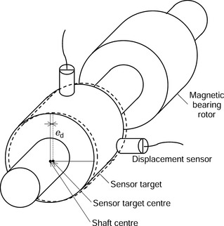
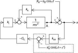
Figure 3.28 shows a definition of eccentric displacement. The sensor target centre is displaced from the shaft centre by ed. The detected sensor outputs include position errors, so that
In this situation, the shaft is suspended at the centre position but the target ring is not rotating about the shaft axis so that the sensor has a target eccentric displacement. Figure 3.29 shows the x-axis block diagram including the influence of the displacement errors for x-axis. At the output of the magnetic bearing displacement, Xe is added so that the sensor feedback signal includes the position error. A simplification of this block diagram provides a transfer function of x/Xe:
From this transfer function the following facts are obvious:
(a) At low rotational speed, the transfer function is (−kx)/(kiksn − kx). Hence the disturbance can be suppressed.
(b) At high rotational speed, the transfer function is unity. Therefore the sensor output includes the sinusoidal variation of the error (with amplitude ed).
If the magnetic bearing rotor has a misalignment from the shaft centre then eccentric displacement Xe is added to the point A in Figure 3.29. In this case, radial force is generated by the displacement-force factor.
Draw the transfer function of x/Xe. Obtain the waveforms of the displacement and the negative feedback force for ed = 10 μm.
Figure 3.30(a) shows an example of the transfer function of x/Xe. The controller has an integral control so that the transfer function is quite low at low frequency. At about 1200 rad/s, the transfer function is more than 0 dB so that the sensor output is more than ed. At 2400 rad/s it reaches a peak value of 10 dB then it decreases to 0dB. The phase angle varies with frequency; it is 90 deg at low frequency then gradually delays to 360 deg at high frequency.
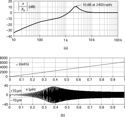
Figure 3.30(b) shows the result of acceleration. The shaft speed is increased from 0 to 60 000 r/min as a ramp function. The amplitude of Xe is constant at 10 μm. The displacement x is small at low speed; however, at about 2400 rad/s, the amplitude is about three times Xe, corresponding to 10 dB of the amplitude of x/Xe. The amplitude then gradually decreases to 10 μm, i.e., ed. The current ix characteristic is similar to the displacement x so that considerable high frequency current is required.
As shown in the previous section, higher frequency current is also eliminated by the synchronized disturbance elimination. In addition, a simple elimination method is shown by the dotted lines in Figure 3.29. If the eccentric displacement is known then a signal injection of ed × cos(ωt + φ*) to the sensor output is effective. The amplitude e*d and the phase angle φ* are adjusted to the actual values to eliminate the influence.
3.6 Synchronized displacement suppression
In section 3.4, a synchronized disturbance elimination method was introduced. The elimination method detects disturbance components synchronized with rotor rotation and then subtracts the detected components from the radial displacement signals so that in the frequency characteristics the loop gain had a dip at the rotor rotational frequency where feedback forces and currents are significantly reduced. However, this does not suppress the radial displacements significantly.
In some applications, the shaft radial position should be forced to zero or to be as small as possible. If the frequency characteristics of the loop transfer function have a peak at the rotor rotational frequency then the rotor displacement can be reduced. Feedback forces and currents are required for displacement suppression. These have to be increased for precise positioning.
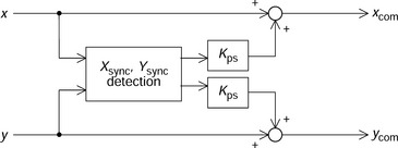
Figure 3.31 shows a block diagram for the required signal conditioning. The inputs are the radial displacements x and y. From these signals, synchronized components Xsync and Ysync are detected as written in (3.37). These detected synchronized components are amplified by Kps and then added to the radial displacements to obtain xcom and ycom. Note that synchronized components are not subtracted as in the elimination method, instead, these are added to the displacements. If Kps is increased then xcom and ycom include Kps-scaled synchronized components. The gain increase at the rotor rotational frequency enhances the loop gain. The synchronized components are amplified in the PID controllers so that radial force commands are generated to reduce the radial displacements. Hence this method is valid at low speed range where PID controllers and current drivers can provide enough suppression current.
Show the effectiveness of enhanced stiffness at a rotational speed of 1200r/min. Consider the influence of both an unbalance of meε = 10−6 and a 1 μm misalignment of the sensor target ring. Then show the acceleration characteristics. Discuss the characteristics of the adding and subtracting methods for the synchronized components.
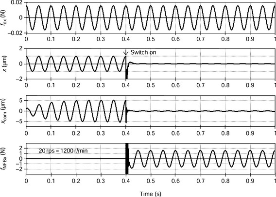
Figure 3.32 shows waveforms to illustrate the effectiveness of the synchronized displacement suppression. The rotor is rotating at a constant speed of 1200 r/min. Two causes of disturbance are included, one is an unbalance of meε = 10−6 and the other is a sensor target ring offset of 1 μm. The suppression is switched on at a time of 0.4 s with Kps = 10. The waveforms are for an unbalance force fdx, x-axis radial displacement, compensated radial displacement xcom and negative feedback force fNFBx. Before switch-on, the radial displacement has fluctuations; however, the negative feedback force is small. After switch-on, x is significantly reduced and there is an increase in the negative feedback force. However, a large current is injected to generate high radial force in order to suppress the synchronized components of the radial displacements.
During acceleration tests the following are observed:
(a) The subtraction method in section 3.4 is effective only at high rotational speed above the critical speed. The advantage of this method is that the negative feedback current is reduced at high rotational speed.
(b) The adding method in section 3.6 is effective only at low rotational speed under the critical speed. The radial displacement is reduced although high current is required.
(c) Without the subtraction and the addition, the magnetic suspension is stable over the whole speed range. However, the displacement is high at low speed and high current is required at high speed.
It has been shown that synchronized component suppression and elimination should be adjusted depending on the rotor speed and critical speed to take advantage of these controllers. These controllers do not require information about the amplitude and direction of the unbalance and displacement of the sensor target ring and the magnetic bearing rotor. If these can be identified then compensation can be carried out by feed-forward controllers.