
Analysis in rotational coordinates and magnetic suspension strategy for bearingless drives with 2-pole and 4-pole windings
In the previous chapter a primitive bearingless motor was analysed. The primitive bearingless motor has a cylindrical rotor without permanent magnets or squirrel cage conductors so that rotational torque is not generated. The analysis of the primitive bearingless motor is similar to the bearingless motor though it only acts as a radial magnetic bearing; but it is helpful in developing the theory for the bearingless motor.
In this chapter vector control theory for permanent magnet motors is introduced; this theory is also called field-oriented control theory. It derives torque and current relationships using the instantaneous rotational position of the revolving magnetic field [1]. In short, rotational torque is generated by an interaction of the revolving magnetic field and the component of MMF that is perpendicular to the field on the d–q axes. The principle is also applicable to field-excited synchronous machines and induction motors. In addition to the basic principles of operation, rotational speed and torque regulation strategies are developed. To aid understanding, vector control theory is explained here by first studying the dc motor as an example. After the torque analysis, additional windings are introduced and the radial forces are derived for a dc motor with a 4-pole and 2-pole winding layout. Variables in the stationary coordinates, i.e., the dc motor model, are transformed into rotational coordinates to obtain the relationships for the ac motor. The derived equations are applied to a cylindrical permanent magnet motor and a salient-pole synchronous motor.
7.1 Vector control theory of electrical motors
Vector control theory provides a control strategy to regulate the instantaneous rotational torque in electrical machines. In a dc motor the generated shaft torque is proportional to the armature current so that precise dc current regulation produces torque regulation. However, in ac motors both the amplitude and phase angle of the currents (which are now ac) need to be regulated to control the torque. Hence it is important to study the relationships between torque and current.
Figure 7.1 shows the cross section of a 4-pole dc motor. It has a cylindrical slotted rotor (referred to as the armature in a dc machine) and a stator, which has four magnetic poles and a surrounding yoke. The airgap length between the rotor iron and stator pole faces is small but the gap between the stator yoke and the rotor is large so that the stator poles provide magnetic saliency. The 4-pole magnetic field Ψm may be generated by permanent magnets; however, for the analysis, virtual conductors ‘m’ are defined and currents in these virtual conductors generate Ψm so that the stator poles are excited with the polarities shown by N and S.
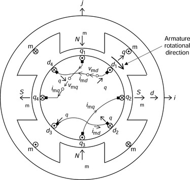
On the armature there are two sets of designated conductors. q1, q2, q3 and q4 are the designated quadrature-axis conductors; the actual conductors rotate but they are connected through brushes and a commutator to the terminals so that the relative angular positions of q1, q2, q3 and q4, with respect to the stator, do not change. This is due to the switching action of the commutator. These conductors are connected in series and are called the q-axis coils because their MMFs sit on the q-axis of the stator poles. Four brushes on the d-axis terminate the armature q-axis coils. Because the conductors are under the stator pole faces, when a positive current flows in q1 a force is generated in the right-hand direction (Fleming’s left-hand rule). Similar forces are generated at the other three conductors so that torque is generated in the clockwise direction. In addition to the q-axis coils another set of conductors are present on the d-axis. These generate an electrically perpendicular MMF with respect to the q-axis conductors. They are also connected in series to form d-axis coils but positive current in these coils does not contribute to torque generation because they are not under the pole faces; however, the amplitude of the 4-pole magnetic field Ψm is increased.
Suppose that the voltage and current applied to the series-connected q-axis coils are vmq and imq respectively, as shown in Figure 7.1. Let us also suppose that the d- and q-axis inductances are Ld and Lq so that
where Rs is the coil resistance, P is the derivative operator with respect to time (= d/dt), ω is the electrical angular frequency, λm is the flux linkage caused by the stator magnetic field and imd is the d-axis coil current. The first term of the equation is the coil resistance voltage drop and the second term is the back-emf due to the coil inductance. The third and fourth terms are described as speed-induced voltages (and can be obtained from the “flux-cutting” rule). For the d-axis coil the voltage vmd is described by
Note that the sign of speed-induced voltage is negative due to the definitions of positive voltage and current direction in the figure. The sign of the speed-induced voltage is described in a later example.
The voltage and current relationships can be written in a matrix form
Instantaneous power pins can be defined as the total instantaneous input power of the system at the terminals so that
Substituting (7.3) into (7.4) yields
The first term is the copper loss in the coils and the second term is the stored magnetic energy in the inductances; these terms do not contribute to torque production. The third term produces reluctance torque, which is generated by a difference between the d- and q-axis inductances due to the magnetic saliency. The fourth term is the excitation torque due to the permanent magnets.
The relationship between the shaft power ps and torque Tr is
where the shaft angular speed ωm is defined as
and pp is the number of pole-pairs. Hence the torque is
The first and second terms are the reluctance and excitation torque respectively.
In vector control theory the torque is expressed as a vector product. Suppose that current vector [i] and flux linkage vector [λ] are defined by d- and q-axis components where
A vector (cross) product of these vectors can be calculated assuming λd = λm + Ldimd and λq = Lqimq so that

Note that this equation corresponds to the derived torque for one pole-pair. Hence we can see that the torque per pole-pair is the vector product of the flux linkage and current. The absolute value of the vector product for torque can be written as
where θ is an angle between [λ] and [i] so that only the current component which is perpendicular to the flux linkage vector contributes to torque production. In the torque controller, the main axis can be oriented on the flux linkage vector, which defines the magnetic field direction, and the quadrature axis is perpendicular to the main axis so that the current component on the quadrature axis is regulated to obtain the required torque. Hence vector control theory is also called field-oriented control theory.
There are several possible strategies for regulating the instantaneous vectors. The voltage and torque equations give an interesting insight, and note that these equations are also valid for permanent magnet synchronous motors as shown in the next section. The regulating strategies for the torque can be summarized as follows
(a) imd = 0 strategy: let the d-axis current be zero. Hence the first term in the brackets in the torque equation is zero so that Tr = ppλmimq. The torque is proportional to the q-axis current when the permanent magnet flux linkage is constant. This simple strategy is often employed in non-salient-pole synchronous motors especially with surface-mounted permanent magnet (SPM) rotors.
(b) Maximizing torque/current ratio strategy: the d- and q-axis currents are determined so that the torque-to-line current ratio is maximized. The current is limited by the motor and inverter current ratings. For the maximum current limit value, torque can be maximized by making imd a function of imq so that both d- and q-axis currents are generated from a torque command. In addition, during low speed operation the copper loss is dominant, hence this strategy results in minimum heat generation.
(c) Power factor = 1 strategy: for the middle-speed range, maximizing the power factor minimizes the product of voltage and current. The power factor of the fundamental voltage and current components (i.e., the cosine of the phase angle as apposed to distortion factor) can be made unity by regulating the d-axis current as a function of imq.
(d) Field weakening strategy: for the high-speed range, the speed-induced voltage due to ωλm may be higher than the rated inverter voltage. The motor terminal voltage can be reduced if the d- and q-axis inductances are relatively high and the d-axis current is negative. This has the effect of reducing the total speed-induced voltage. It is advantageous if Ld is less than Lq (as is the case with interior permanent magnet (IPM) motor, where q-axis saliency is present) so that only low imd is required to weaken the field. Also the subsequent reluctance torque will contribute to the torque production.
The effectiveness of these strategies is dependent on machine parameters Ld, Lq and λm. In addition, these strategies can be chosen to match the rotational speed and torque operating point.
In Figure 7.2 two conductors are rotating in a magnetic field of flux density B. The rotational velocity of the conductors is ωlc; (a) shows the top view and (b) shows the side view. Answer the following questions.
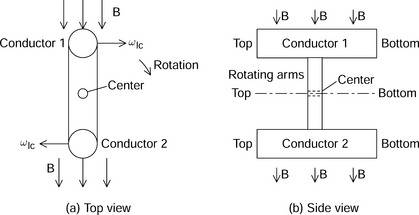
(a) What is the speed-induced voltage polarity in conductors 1 and 2?
(b) If the bottom terminals of conductors 1 and 2 are connected together, what is the voltage polarity of the circuit?
(c) After conductors 1 and 2 are connected, the voltage polarity and current direction are defined for motoring operation, i.e., positive current flows down the second conductor and up the first, while the voltage at the top of the second conductor is positive with respect to the first. Show the polarity of the speed-induced voltage.
(d) For the case when the voltage polarity is reversed with respect to the motoring operation, show the polarity of speed-induced voltage.
(e) Suppose that the conductors are composed of several series-connected wires so that a coil is formed and flux is generated by current in another coil on the d-axis having a self-inductance Ld. The electrical rotational angular speed is ω. The voltage polarity and current direction of the q-axis coil are as in Figure 7.1. Draw a side view for the conductors q1 and q4. Show the speed-induced voltage due to the d-axis coil and also show the speed-induced voltage due to the d-axis permanent magnets.
(f) Draw a side view for the d-axis conductors d1 and d4 of the d-axis coil in Figure 7.1 and show the speed-induced voltage.
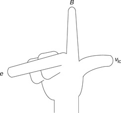
The polarity of the speed-induced voltage is defined using Fleming’s right-hand rule as shown in Figure 7.3. The thumb, forefinger and middle finger indicate the directions of speed vlc, flux density B and induced voltage e.
(a) The voltage potential of the bottom terminal 1B of conductor 1 is positive with respect to the top terminal 1T as shown in Figure 7.4(a) while the voltage potential of the top terminal 2T of conductor 2 is positive with respect to the bottom 2B, again as shown in Figure 7.4(a).
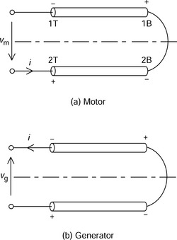
(b) The top of the conductor 2 is positive with respect to the top of conductor 1 as shown in Figure 7.4(a).
(c) Positive – The induced voltage is opposite to the terminal voltage as shown in Figure 7.4(a).
(d) Negative – The induced voltage has the same polarity as the terminal voltage as shown in Figure 7.4(b). Note that the polarity of the speed-induced voltage is dependent on the voltage definition. Even in the case of a generator, the current direction can be defined in the opposite direction, while voltage polarity is the same as that in a motor.
(e) vmq = ωLdimd + ωλm. Refer to Figure 7.5(a).
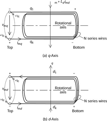
(f) vmd = −ωLqimq. Refer to Figure 7.5(b). The voltage polarity is in the opposite direction to that in Figure 7.5(a). The voltage polarity is based on Figure 7.1.
7.2 Coordinate transformation and torque regulation
In the previous section, torque was expressed as a function of the d- and q-axis currents using a dc motor model. In vector control theory, using rotating reference axes and a 3-phase to 2-phase coordinate transformation, it can be shown that the synchronous and induction motors are equivalent to the dc motor (indeed, in a dc motor, while the armature draws dc current, the current in the actual armature coils is ac with a square-wave shape due to the switching action of the commutator). In this section the relationships between the dc motor and the synchronous motor are shown. The theory of the induction motor is rather more complicated and advanced readers are recommended to refer to Reference [1].
Figure 7.6 shows the cross section of a 2-phase synchronous motor. The rotor has four salient poles and field-winding conductors m are arranged so that 4-pole magnetization is produced. The i- and j-axes are aligned on the magnetic poles. These axes are fixed to the rotor so that they rotate with rotor rotation. The rotor angular position is defined by the angle φ. Note that the direction of rotation is opposite to that in Figure 7.1. This is in order to have corresponding movement with respect to the defined axes. The relative movement between armature and field is the same although in Figure 7.6 the field rotates and in Figure 7.1 the armature rotates. Located in the stator slots are conductors ma and mb which form a 4-pole 2-phase winding. The current directions of conductors ma and mb are defined so that the MMF directions correspond to the d1-d4 and q1−q4 conductors in Figure 7.1 at the point where φ = 0. At this angular position it can be seen that the 2-phase motor in Figure 7.6 is equivalent to the dc motor in Figure 7.1. However, ma and mb are fixed to the stator and are not fed through brushes and a commutator. Hence the relative position of the conductors varies with the rotor angular position. On the other hand, the conductors in Figure 7.1 are stationary because the conductor currents are fed through brushes and a commutator.
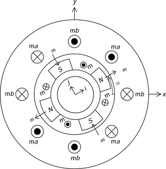
To generate an equivalent MMF distribution, the conductor currents ima and imb can be varied with the rotor angular position using a rotational coordinate transformation matrix, as shown:
The equation matrix shows that the MMF distribution in Figure 7.1 is produced, and that the currents ima and imb are regulated by the d- and q-axis currents and also the rotor angular position φ.
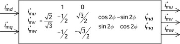
Figure 7.7 shows an example of a winding arrangement in a practical 3-phase motor. On the stator are 24 slots that accommodate the motor conductors, which are indicated by letters and connected so that a 3-phase winding comprising of mu, mv and mw is formed. The current directions are balanced and defined so as to correspond with an equivalent 2-phase ac machine. The currents imu, imv and imw can be related to the equivalent current distribution shown in Figure 7.6 using the transformation
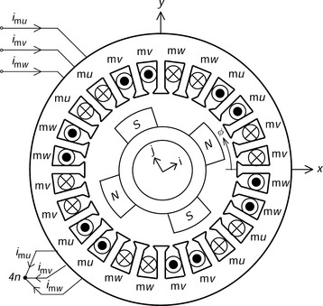

This transformation is the 2-phase to 3-phase transformation matrix. The 2-phase current set has two degrees of freedom whereas the 3-phase current set has three degrees of freedom. However, the sum of the 3-phase currents is zero in the above calculation, whatever the values of the 2-phase currents. Since the current sum at the neutral point 4n is zero, the 3-phase system is a three-wire, three-terminal system with a star connection.
Figure 7.8 shows a block diagram of a control to calculate the instantaneous 3-phase current commands from the d- and q-axis current commands i*md and i*mq. In a vector controller the currents are controlled using the dc machine model.
The dc current commands are generated using the torque demand, the speed, etc. The 3-phase current commands i*mu, i*mv and i*mw are generated using (7.9) and (7.10).
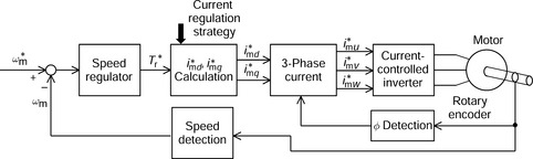
Figure 7.9 shows an example of a speed-regulated motor drive system. On the rotor shaft is a rotary encoder, which is used to detect the instantaneous rotor angular position. The shaft speed ωm is detected and compared with the speed command to generate a speed error. The speed error is amplified by a speed regulator to generate the torque command T*r. Using this command, the d- and q-axis current commands are calculated depending on the current regulation strategy. These current commands are then transformed into the 3-phase current commands. The motor currents are supplied and regulated to follow these current commands by an inverter. In steady-state conditions, the rotor runs at a constant speed with a constant load torque so that the torque command is equivalent to the load torque. The d- and q-axis currents are dc values whereas the 3-phase currents and their associated commands are 3-phase sinusoidal waveforms.
7.3 Vector control theory in bearingless motors
In the previous section, vector control theory was briefly explained using a dc machine model. This model was defined using conductors fixed to the rotor so that the dc machine model can be described in a rotational coordinate system model. In this section a rotational coordinate model of a 4-pole and 2-pole bearingless motor is introduced and the basic relationships between the flux linkages, currents and suspension forces are derived [2].
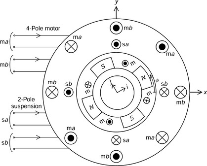
Figure 7.10 shows a bearingless motor with 4-pole motor windings md and mq and 2-pole suspension windings sd and sq, as well as the motor field winding m. The motor and suspension currents are rotor-mounted and fed through a commutator and brushes (which are not shown in the figure). The rotor is rotating in a counter-clockwise direction although the relative position of conductors is stationary with respect to the stator. Windings m, md and mq are motor windings corresponding to those in Figure 7.1. Conductors sd and sq are added as the suspension windings.
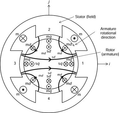
For the first step of the suspension force generation analysis, an inductance matrix has to be derived. The mutual inductances between the 4-pole and 2-pole windings play an important role in suspension force generation, and these mutual inductances should be represented as a function of the radial rotor displacement.
Figure 7.11 shows flux distributions when a rotor is displaced from the centre position. In Figure 7.11(a) the rotor is displaced in the i-axis direction. The 4-pole flux distribution generated by winding m is unbalanced so that more flux is concentrated under stator-pole 1. Hence some flux mutually links winding sd. Note that the flux linkage is in the same direction for both windings. Let us assume that the flux linkage is proportional to the rotor displacement; the flux linkage between the m and sd windings can then be expressed as λ′mi, where λ′m is a suspension force constant (Wb/m) and i is the i-axis rotor displacement. Similar flux linkage occurs when winding md is excited. In this case the mutual inductance is expressed as M′di, where M′d is a suspension force constant (H/m). A similar characteristic also occurs for the j-axis rotor displacement.
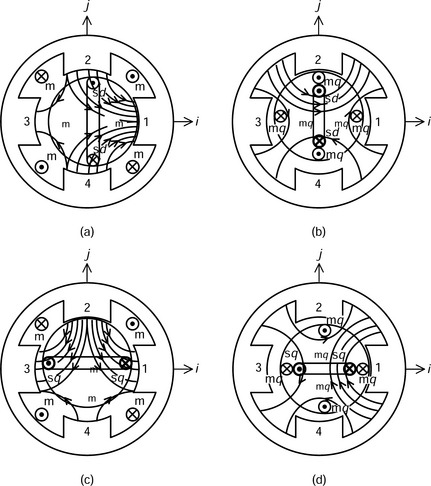
Figure 7.11 Mutual couplings when a rotor is displaced: (a) m-excited flux links to sd; (b) mq-excited flux links to sd; (c) m-excited flux links to sq; (d) mq-excited flux links to sq
Figure 7.11(b) shows the flux distribution with winding mq excited. Suppose that the rotor was originally positioned at the stator centre producing a 4-pole symmetrical flux distribution. In that case some positive-direction flux flows around stator-pole 2 and links winding sd; however, negative flux around stator-pole 4 also links with winding sd so that the sum of the net flux linkage is zero. But when the rotor is displaced along the j-axis the positive flux is increased and the negative flux is decreased. Hence the flux linkage is no longer zero, so a mutual inductance exists between the mq and sd windings, which is expressed as M′qj, i.e., the product of suspension force constant M′q (H/m) and the j-axis displacement.
Figure 7.11(c,d) shows the variation of the rotor position in the same two directions, and these also lead to mutual inductances with winding sq. Figure 7.11(c) illustrates the case when a rotor is displaced in j-axis direction. The mutual inductance between the m and sq windings is expressed as −λ′mj, where j is the j-axis radial rotor displacement. The mutual inductance is negative because the flux linkage is reversed with respect to the polarity of the sq winding. Figure 7.11(d) illustrates the mutual inductance between windings mq and sq.
The mutual coupling of the suspension and md windings is the same as with the field winding since the md winding has the same MMF space distribution. The relationships between flux linkage and winding currents can be expressed in a matrix form
where λmd, λmq, λsd and λsq are flux linkages of the motor and suspension d- and q-axis windings and λ′m (Wb/m), M′d (H/m) and M′q (H/m) are the suspension force constants.
Using this matrix equation, the stored magnetic co-energy W′m can be derived (neglecting magnetic saturation). If saturation does not exist then W′m is equal to the stored magnetic energy Wm so that
Substituting (7.11) into (7.12) yields
Although the equation is based on a non-holonomic system with only rotational movement, the derived suspension forces are valid because these forces are obtained from partial derivatives with respect to radial displacements. Hence the suspension forces are
These equations can be written in a simple matrix form as
Note that this matrix equation is similar to the one derived in section 6.6 for the primitive bearingless motor with a cylindrical rotor. The i- and j-axis suspension forces are proportional to suspension currents and the coefficients λ′m + M′dimd M′qiMq and, where λ′m is the derivative of the flux linkage due to the main field with respect to the radial rotor displacement and M′dimd and M′qimq are derivatives of d- and q-axis winding flux linkages with respect to the radial displacement. Hence the suspension force characteristics of bearingless motors can be determined using the suspension force constants λ′m, M′d and M′q.
For a cylindrical rotor, M′d and M′q are equal in value so that the matrix equation can be simplified. This is the case for the SPM motor. If thick magnets are used then M′dimd and M′qimq can also be neglected (with respect to λ′m) leading to further simplification. For an inset type of permanent magnet rotor (which has saliency on the magnet q-axis) with thick magnets, only M′dimd can be neglected because of the low d-axis permeance.
In some cases, motors with interior permanent magnet rotors may have parameters λ′m, M′d and M′q which vary depending on the d- and q-axis motor current values because of magnetic saturation in some parts of the rotor core (such as the rotor pole faces). In these cases, parameter identification is the key to successful magnetic suspension since they are functions of the current.
In induction motors, λ′m is zero since there is no field excitation. In addition M′d and M′q are equal because the rotor is cylindrical. The d-axis current is the excitation current and the q-axis current is the torque-generating current. In synchronous reluctance motors also λ′m is zero. Hence it can be seen that the suspension force equation governs the suspension force and current relationships in many types of bearingless motor which have 4-pole motor windings and 2-pole suspension windings.
7.4 Coordinate transformation from dc to ac bearingless machines
In the previous section the suspension force and current relationships were derived for a dc machine with 4-pole and 2-pole windings. In this section current regulating strategies with rotational and 2/3-phase transformations are shown and basic radial positioning schemes with indirect and direct vector controllers are introduced.
Figure 7.12 shows the structure of a 2-phase ac bearingless machine. This figure is similar to the 2-phase ac machine shown previously in section 7.2; however, the 2-pole windings sa and sb have been added. There are four series-connected windings with eight terminals as illustrated. sa and sb correspond to the sd and sq windings in Figure 7.10. The stator conductors are located in slots in the stator and there is an internal rotor. Two perpendicular axes, x and y, are arbitrarily fixed to the stator so that the radial position relationships between the i- and j-axes and the x- and y-axes are defined by
Similar relationships are also defined for the suspension forces so that
The 4-pole current relationships between ima, imb, imd and imq were previously given in (7.9). The 2-pole current relationship can also be defined:
Figure 7.13 shows an example of an actual 3-phase ac bearingless machine. The 4-pole conductors correspond to the 3-phase conductors as shown previously in section 7.2; however, there are additional 2-pole conductors in the stator slots to generate the suspension forces. The 2-pole conductors are su, sv and sw. The transformation between the 2-phase and 3-phase current representations was given in (7.10) for the 4-pole case. The same transformation exists for the 2-pole currents
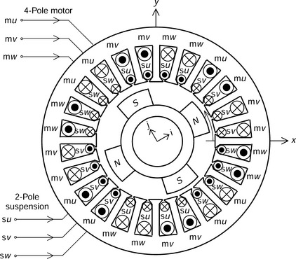
There are six terminals for the two sets of 3-phase windings. However, two neutral points are formed – one is for mu, mv and mw and the other is for su, sv and sw (although these are not shown in the Figure 7.13).
Let us derive a relationship between the suspension forces and winding currents. Substitute (7.18) into the left-hand side of (7.16); an expression for (isd, isq)t can be derived from (7.19) and (7.20) which can be substituted into the right-hand side of (7.16). Solving for suspension forces yields
Note that this matrix equation shows the relationship between the suspension forces in the stationary coordinates as a function of the suspension winding currents. It can be seen that the suspension forces are also functions of the rotor angular position and suspension force constants.
An insight into the current regulating scheme can be obtained from the above matrix equation. Let us suppose that the suspension force constants and rotor angular position are known so that the 3-phase current commands i*su, i*sv and i*sw are generated from the suspension force commands F*x and F*y.
This matrix equation provides the basic operation of a decoupling controller. For the radial position regulating loops, suspension force commands are required in the stationary frame so that the winding current commands are controlled. Hence the actual suspension forces correspond to the force commands. The above equation provides a calculation method for the suspension winding currents so that the actual suspension forces follow these commands.
In order to execute the above calculation in a controller, information about the instantaneous d- and q-axis motor currents and the rotor angular position is needed. Figures 7.14 and 7.15 show some possible system block diagrams for the bearingless motor. Figure 7.14 shows an indirect system structure. The decoupling controller executes the above matrix equation. The d- and q-axis current commands generated in the motor controller are used in the decoupling controller, assuming that the actual d- and q-axis motor currents follow these commands. This system structure is useful when the motor and decoupling controllers are built into one digital processor.
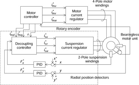

Figure 7.15 shows a direct system structure. In the direct system, the d- and q-axis motor currents are detected from the instantaneous line currents so that these currents are used in the decoupling controller. There is no signal link between motor and decoupling controllers. Hence this system is suitable in the case where the motor is driven by an independent inverter. This structure is good for applications where the motor is driven by a low-cost general-purpose inverter. These are now widely available.
7.5 System block diagrams of bearingless machines
In this section, system block diagrams are introduced which are based on the relationship between the suspension force and the associated winding currents as derived in the previous section. The block diagrams are drawn for a few basic synchronous motor structures, i.e., an SPM motor, a salient-pole permanent magnet motor and a synchronous reluctance motor.
In the cylindrical-rotor synchronous motor such as the SPM motor, there is no magnetic saliency so that the shaft torque is written as Tr = ppλmimq. Since d-axis current does not contribute to the torque production, the motor controller sets imd = 0. In addition, armature reaction is not apparent since the flux linkage, which originates from winding inductances, is small compared to the permanent magnet flux linkage when thick permanent magnets are employed. Hence λ′m ![]() M′qimq and M′dimd = 0. Substituting these relations into (7.22) results in a simple matrix calculation
M′qimq and M′dimd = 0. Substituting these relations into (7.22) results in a simple matrix calculation
Figure 7.16 shows a block diagram for the SPM bearingless motor. The suspension force commands F*x and F*y are generated from the radial position regulators using the detected radial shaft position. The decoupling and 2-phase/3-phase blocks generate 2-pole suspension winding current commands using the above equation. A current regulator, i.e., a current-controlled inverter, regulates the 3-phase currents. In a motor speed controller, the rotational speed and angular position are detected. The detected speed is compared with its command and a torque command is generated via the speed regulator. Using this, the q-axis motor current command is generated. Note that the d-axis motor current command is zero. The 2-phase and 3-phase current commands are generated and a current regulator provides instantaneous current regulation of the motor winding currents. The radial position controller requires only λ′m and not M′dimd and M′qimq, so the d- and q-axis motor current values are not required.
In the salient-pole synchronous machine, the structure of the system block diagram is rather complicated. The inverse matrix shown in (7.22) can be simplified to
where
and the current commands are defined by
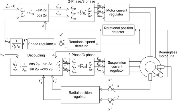
Figure 7.17 shows a block diagram for the salient-pole PM motor. The blocks corresponding to (7.25) and (7.26) are added and the function for the decoupling controller is modified to include θf.
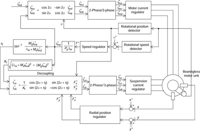
Figure 7.17 An indirect system configuration of a salient-pole bearingless motor with armature reaction compensation
Figure 7.18 shows a direct type of system configuration. The d- and q-axis motor currents are detected using the measured 3-phase line currents, then Kf and θf are generated in blocks corresponding to (7.25) and (7.26). Note that the motor-drive inverter is operating independently of the radial-position-regulating loops. Flux density detectors, e.g., Hall sensors or search coils, can also be integrated in motor airgap, and then, these sensors provide Kf, θf and φ. The detailed system requirements and machine parameter measurements, as well as detection methods, are described in a later section.
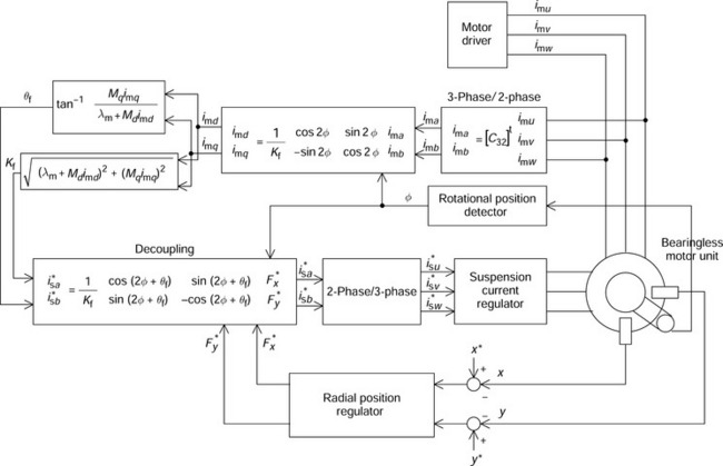
Figure 7.18 A direct system configuration of a salient-pole bearingless motor with armature reaction compensation
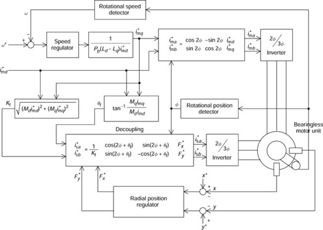
Figure 7.19 shows the block diagram for a synchronous reluctance type of bearingless motor. In synchronous reluctance motors there is no permanent magnet excitation so that λm in the torque equation is zero and λ′m in the suspension force equation is also zero. The q-axis motor current command block and the Kf and θf blocks are modified. Detailed requirements for synchronous reluctance bearingless motors will be described in a later chapter.
References
[1] Novotny, D.W., Lipo, T.A., “Vector Control and Dynamic of AC Drive”. Oxford University Press, Oxford, 1996. [ISBN 0198564392].
[2] Chiba, Akira, Deido, Tazumi, Fukao, Tadashi, Rahman, M.A., “An Analysis of Bearingless AC Motors”. IEEE Transaction on Energy Conversion, Vol. 9, No. 1, 1994:61–68. [March].