
Switched reluctance bearingless motors
In this chapter the bearingless switched reluctance motor is introduced. Conventional switched reluctance motors with mechanical bearings have generated significant interest among researchers and industrial engineers. For particular environments and applications, the switched reluctance motor can have superior performance because of its inherent features such as being fail-safe, robustness, low cost and possible operation at high temperature or in intense temperature variation [1–7]. Industrial drives which utilize the switched reluctance machine have been available for some time.
The switched reluctance motor also offers the possibility of operation as a bearingless motor. Torque is generated by magnetic attraction between rotor and stator poles. In this process a significant amount of attractive radial force is generated because the switched reluctance motor has salient poles and a short airgap length between these poles in order to effectively produce a reluctance torque. It is quite possible to take an advantage of the inherent high radial force that is produced for rotor shaft magnetic suspension. Therefore bearingless switched reluctance motors with differential stator winding configurations have been developed [8–14]. These motors have motor windings and suspension windings wound in the same stator in order to produce a suspension force that can realize rotor shaft suspension. Hence these motors are expected to be suitable for maintenance-free drives used in special circumstances such as high temperature, wide temperature variation and high acceleration operation.
15.1 Configuration of stator windings and principles of suspension force generation
Figure 15.1 shows only the A-phase stator winding of a 3-phase system with additional differential windings. The motor winding Nma consists of four coils connected in series while the suspension windings Nsa1 and Nsa2 consist of two coils each. These coils are separately wound around the top of opposite stator poles. The B-phase winding configuration is located at 30 mechanical degrees to the A phase, and the C-phase winding configuration is located at 60 mechanical degrees to the A phase. The axes a1 and a2 of a perpendicular coordinate system can be defined using the A-phase winding as a reference, as shown in Figure 15.1. In this case, the axes x and y are aligned with a1 and a2 respectively. Similarly, the axes of coordinates b1, b2, c1 and c2 can be defined for the B-phase and C-phase windings. Since the number of stator poles is 12, the step angle is 15 mechanical degrees. The rotor angular position φ is defined as φ = 0 when aligned with the A phase. The rotor angular position φ in Figure 15.1 is −π/18 (−10 deg).
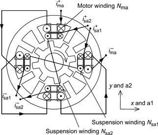
Figure 15.2 shows the principle of suspension force generation for the bearingless switched reluctance motor. The thick solid lines show the symmetrical 4-pole flux produced by the 4-pole motor winding current ima. The broken lines show the symmetrical 2-pole flux produced by the 2-pole suspension winding current isa1. In this situation, the flux density in air-gap section 1 is increased because the direction of the 2-pole flux is the same as that of the 4-pole flux. In contrast, the flux density in airgap section 2 is decreased since the direction of the 2-pole flux is opposite to that of the 4-pole flux. Therefore, superposition of the airgap magnetic flux waves results in a suspension force F acting along the x-axis. A negative suspension force along the x-axis can be generated with a negative current isa1. A suspension force on the y-axis can be produced using a 2-pole suspension winding current isa2. Hence a suspension force can be generated in any desired direction by a vector sum of these forces. It should be noted that the 4-pole flux produced by the motor winding currents is essential as the bias magnetic flux for suspension force generation. So far only one main and suspension winding has been considered; however, this principle can be applied to the B- and C-phases so that a suspension force can be continuously generated by these three phases in turn for every 15 deg, i.e., from the start of the switching overlap up to the aligned position (turn-off).
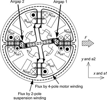
If rotor and stator poles are aligned, a high suspension force is generated. As the rotor rotates away from the aligned position the suspension force becomes less because of the increase in magnetic reluctance causing a decrease in airgap flux (for constant phase current). The relationships between suspension force and stator winding currents are found to be dependent on the rotor angular position; so for successful magnetic suspension, the force must be controlled at all rotor angular positions. Therefore it is essential to derive an accurate theoretical algorithm of the suspension force for successful control because these formulae are required to maintain constant loop gain in the controller when using a negative feedback loop.
15.2 Derivation of inductances
Figure 15.3 shows the magnetic equivalent circuit for the A phase only. Voltage sources represent the MMFs of the 4-pole motor windings and the 2-pole suspension windings and, in addition, the magnetic permeances of air gap are represented by electrical conductances. The definitions of the variables in Figure 15.3 are as follows: Nm is the number of turns of the motor winding, Ns is the number of turns of the suspension winding, Pa1−Pa4 are the permeances of the airgap under the A-phase winding poles and ψa1−ψa4 are the magnetic fluxes of each pole. Only the A-phase magnetic equivalent circuit is used in the simple calculation in this section. This is possible because the switched reluctance motor has little mutual inductance between phases.
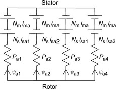
If each of the permeances (shown as Pa1 to Pa4) can be simply assumed, the self inductances and the mutual inductances of each winding of the A phase can be calculated from Figure 15.3. The self inductances and the mutual inductances can be written as [9]:
15.3 Assumption and calculation of permeances
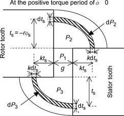
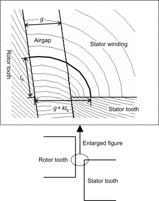
The gap permeance Pa1 of the airgap section 1 can be divided into three permeance components P1−P3 as shown in Figure 15.4; this is an enlargement of Figure 15.2. P1 can be derived with straight magnetic paths while P2 and P3 can be derived with the assumed (as illustrated) magnetic paths. The variables in Figure 15.4 can be defined as follows: r is the radius of the rotor pole, g is the airgap length, ts is a position on the circular surface (outer radius) of the rotor pole, φs is an angle of ts in polar coordinates, dts is the derivative of ts, and dP2 and dP3 are the permeances of the assumed infinitesimal-width magnetic paths. The following assumptions are considered in calculating the permeances:
1. Magnetic saturation is neglected. A calculation for suspension force and torque under magnetic saturation is given in [10] for advanced readers.
2. The square of rotor displacement is small compared with the square of airgap length.
3. Flux paths which do not link the rotor are neglected.
4. Flux paths between stator poles and rotor inter-polar area are neglected.
5. Only fringing fluxes at the aligned position can be neglected because the airgap length is very short.
Figure 15.5 shows an enlargement of the magnetic paths at the pole edge obtained from a two-dimensional finite element analysis. The shape of the fringing magnetic paths is elliptical so that the fringing magnetic paths of the permeances P2 and P3 can be assumed to follow elliptical curves using a variable k. If the semi-minor axis of the elliptical curve is ts, the semi-major axis can be expressed as g + kts.
It is important to evaluate the value of constant k to determine the shape of the ellipse. k can be calculated from each magnetic path in Figure 15.5. Figure 15.6 shows the relationship between k and ts as derived from results of the finite element analysis. This analysis is carried out with airgap lengths of 100, 220 and 300 μm in order to observe the dependence of the fringing fluxes on the airgap length.
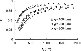
It can be seen that the relationship between k and ts is dependent on the airgap length g. Therefore a general expression between k and ts in terms of g should be derived. Figure 15.7 shows the relationship between k and ts/g, and k is found to be a function of only ts/g.
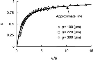
From Figure 15.7, the relationship between k and ts/g can be approximated to
where a is a constant calculated, using the method of the least squares, to be 1.18. The average cross section area S of dP2 and dP3 can be expressed as:
where h is the iron stack length. Assuming that l is the magnetic path length of the permeances dP2 and dP3, l can be approximated to [10]:
Consequently, the permeances dP2 and dP3 can be derived from (15.7), (15.8) and (15.9) so that
where μ0 is permeability of the air. The suspension force is proportional to the derivative of the gap permeance with respect to the rotor displacement. It is necessary to take into account the rotor displacement in the expressions for the airgap length g as used in the expression for permeance Pa1; hence we can write
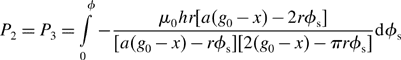
where g0 is the average airgap length, x is the rotor displacement on the x-axis. Therefore P2 and P3 can be derived from (15.10) and (15.11) using the equation
The permeance P1 of the airgap between the rotor and stator poles can be simply derived as
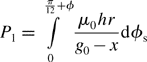
The theoretical formula of the gap permeance Pa1 during the positive torque period of φ ≤ 0 can be derived from (15.12) and (15.13) so that:
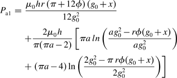
provided that x2 can be neglected. This should be the case because g0 is large compared to x. Similarly, the theoretical formulae of the gap permeances Pa2 to Pa4 can also be derived.
15.4 Theoretical formulae of suspension force and torque
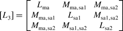
The self and mutual inductances can be derived by substituting gap permeances Pa1 to Pa4, calculated from the above method, into (15.1) to (15.6). It is possible to construct a 3 × 3 inductance matrix [L3] from the derived self and mutual inductances. The inductance matrix [L3] of phase A can then be written as
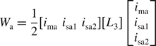
Next, the stored magnetic energy Wa in phase A can be expressed using (15.15) so that
The suspension forces Fx and Fy produced by the current in phase A can be obtained from the derivatives (with respect to rotor displacements x and y)of the stored magnetic energy Wa. This leads to expressions for the suspension forces, as derived from (15.16):
The proportional coefficient Kf (φ) is a function of the rotor angular position φ and the dimensions of the motor. There are two different expressions for this depending on the torque. It becomes Kfp(φ) when there is positive torque (φ ≤ 0), where
This is correct when the rotor radial position is under stable control at the centre of the stator bore, i.e., x and y are zero. On the other hand, it is equal to the coefficient Kfn (φ) when there is negative torque (φ > 0), where
The first term in the square brackets of (15.19) and (15.20) is due to the straight magnetic paths across the airgap between the rotor and stator poles so that the first term is dominant. This decreases linearly as the rotor rotates away from the aligned position. At φ = ±15 deg, i.e., at the start of overlap position, the first term becomes zero. However, a suspension force is generated by the second term which is due to the fringing magnetic paths (which are assumed as elliptical lines as shown earlier). Therefore the second term plays an important role during the overlap.
Similarly, the suspension forces due to phases B and C can be derived. The suspension forces along axes a1, a2, b1, b2, c1 and c2 can be obtained:
1. During the conduction period of phase A(−15 deg ≤ φ< 15 deg)
2. During the conduction period of phase C (0 deg ≤ φ< 30 deg)
3. During the conduction period of phase B (15 deg ≤ φ< 45 deg)
A suspension force can be continuously generated by the switching of phases A, B and C using (15.21) to (15.23). As a result successful magnetic suspension can be realized for all rotor angular positions.
The torque Ta due to phase A can be written as
The second and third terms in the parenthesis are due to the suspension winding currents. The proportional coefficient Gt(φ) is again a function of the rotor angular position φ and the dimensions of the motor. During the positive torque period (φ ≤ 0) it becomes
(under stable control at the central position) and during the negative torque period (φ > 0) it is modified to:
15.5 A drive system
In this section a drive system which controls the average torque and instantaneous suspension force to produce stable operation is discussed [11]. This is done by means of controlling the advanced angle of the conduction period of the stator winding currents under any torque condition from no load to full load.
15.5.1 Basic concept of a drive system
The phase-advance angle θm is the angle from the mid-point of the square-wave current conduction period to the aligned position of rotor and stator poles as shown in Figure 15.8. If θm is fixed at π/24 (7.5 deg) for example, the conduction period of phase A is fixed from −15 to 0deg and positive torque is produced. We can use the magnitude of the current to vary the torque (where θm is constant), in which case the amplitude of motor winding currents im has to be zero at zero torque. However, total stable operation cannot be realized since the suspension force requires a motor winding current, i.e., im ≠ 0, even if there is a large suspension winding current. Therefore, it is particularly important for stable operation to bias the magnetic fluxes sufficiently with a non-zero im over the whole torque range. Generation of the bias magnetic fluxes can be realized by controlling θm (rather than controlling the torque solely via the current amplitude).
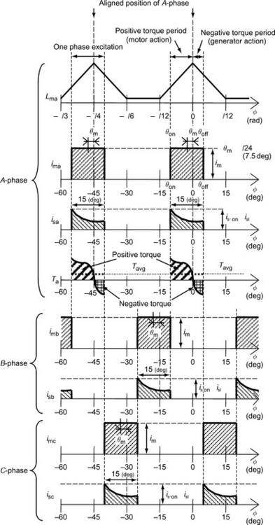
Figure 15.8 shows the idealized current and instantaneous torque waveforms for the drive system. Here isl is the limit of the suspension winding current. The motor winding current im has a square waveform for system simplification. Both the motor winding and the suspension winding currents are simultaneously excited even during the negative torque period by reducing θm from the maximum value of π/24 (7.5 deg). Hence the bias magnetic flux required for generating suspension force is always produced by im. At no load (Tavg = 0), θm becomes zero and the positive torque is equal to the negative torque. The desired average torque Tavg and instantaneous suspension force F can be produced by determining the correct values for θm and im. In the case of a motoring action, θm can be in the range indicated by Figure 15.8 where
If rotor and stator poles are aligned, the suspension force is high. As the rotor moves away from the aligned position the suspension force becomes less because of the increasing magnetic reluctance. Accordingly, the suspension winding current has a maximum value is.on at the turn-on angle θon as shown in Figure 15.8. This is because θon corresponds to the most unaligned position during the conduction period. It is necessary for is.on to be below the limit value isl when determining the advanced angle θm. It was reported in [12] that the optimal conduction period is 15 deg, i.e., one phase excitation, so that the average torque is regulated with square-wave currents in motor windings. It is necessary to reduce θm until the suspension winding current is.on is below the limit value isl. At the same time the motor winding current im should be increased in order to generate the desired average torque Tavg (which will also increase the suspension force).
15.5.2 Drive system structure
The desired values of θm and im, which can simultaneously produce the desired Tavg and F, can be calculated by means of deriving the relationship between Tavg and F with respect to θm and im from (15.17), (15.18) and (15.24). It is necessary to include the condition that θm is a maximum value for the following reasons:
1. It minimizes the negative instantaneous torque.
2. The maximum positive torque necessary for the desired Tavg can be reduced.
However, it should be remembered that the suspension winding current is.on at the turn-on angle θon should be below the limit value isl. Based on these considerations, the motor winding current im is determined from average torque and suspension force commands [11].
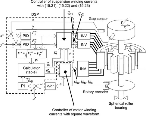
Figure 15.9 shows the structure of a suitable drive system. The calculator for controlling θ*m and i*m is added to the system with a negative feedback loop. The calculator consists of a look-up table with outputs for θ*m and i*m for corresponding inputs of T*avg and F*. The table is written in order to reduce the sampling time of the digital signal processor. The controller of the suspension winding currents uses (15.21), (15.22) and (15.23). It can be seen that the controller of motor main winding currents is separate from the digital signal processor. Therefore it is possible to realize a high-speed drive without a time delay in the control cycle of motor winding currents.
15.5.3 Experimental results
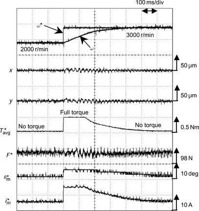
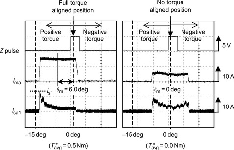
A test machine was built as shown in Figure 15.9. The bottom of the rotor shaft is held by a spherical roller bearing and it is connected to the load machine through a torque meter. The radial rotor position is controlled in two perpendicular axes x and y. A weight hangs via a pulley which pulls the shaft along the negative x-axis to apply a suspension force F = 73.5 N. The dimensions of the test motor are shown in Table 15.1. Figure 15.10 shows the waveforms of rotational speed ω, rotational speed command ω*, rotor displacements x and y, average torque command T*avg, suspension force command F*, advanced angle command θ*m, and finally motor winding current command i*m, for a step change in speed reference of the drive system from 2000 to 3000 r/min. Figure 15.11 shows the waveforms from the Z pulse in the rotary encoder (giving angular position), the A-phase main winding current ima and the A-phase suspension winding current isa1 when T*avg = 0.5 and 0.0 Nm. During full-torque acceleration, θ*m and i*m are increased in order to produce maximum torque. Before and after the acceleration when the torque is low, the suspension-force bias flux is still generated by the im at θ*m = 0 and the operation of the bearingless switched reluctance motor is still stable despite the sudden step acceleration. Hence the drive system can realize stable operation by means of controlling θm and im under any torque condition from no load to full load.
Table 15.1
| Number of turns of motor main winding, Nm (0.8 mm φ, 3 parallels, 1.51 mm2) | 14 turns |
| Number of turns of suspension winding, Ns (0.8 mm φ, 2 parallels, 1.01 mm2) | 11 turns |
| Arc angle of rotor and stator teeth | 15 deg |
| Stack length, h | 50 mm |
| Outside diameter of stator core | 100 mm |
| Inside diameter of stator pole | 50 mm |
| Radius of rotor pole, r | 24.78 mm |
| Average airgap length, g0 | 0.22 mm |
15.6 A feed-forward compensator for vibration reduction considering magnetic attraction force
Regardless of whether the machine is a conventional or a bearingless switched reluctance motor, rotor eccentricity due to mechanical error causes large radial forces due to the magnetic attraction force. This is a major cause of vibration and subsequent noise emission in switched reluctance motors. In conventional switched reluctance motors, compensation of the magnetic attraction force is not possible (hence they can be noisy). On the other hand, the bearingless switched reluctance motor does generate a controlled radial force. Therefore, it is possible to actively compensate for the radial magnetic force due to rotor eccentricity using the suspension force. The time delay in the compensation is minimized by a feed-forward compensator in the rotor radial positioning. Hence in this section a feed-forward compensator for vibration reduction is discussed.
15.6.1 Relationship between magnetic centre and magnetic attraction force
Rotor displacement (eccentricity) from the magnetic centre of the stator causes non-uniformity in the magnetic flux distribution with a concentration of flux where the airgap is narrowest. Therefore the magnetic attraction force acts in the direction of rotor displacement since the flux density in the airgap is higher at this point. To assess the effects of eccentricity it is necessary to measure accurately the radial position of the magnetic centre. Figure 15.12 shows the measured radial position as a function of rotational direction [13] of the 3-phase machine given in Table 15.1. The rotor centre draws a locus in the shape of a circle with a radius of about 13 μm. The displacement of the rotor from the stator centre gives the direction and magnitude of the required suspension force to bring the rotor back to the centre. Hence the rotor centre and the magnetic centre can be described. The origin for the rotor radial position controller is set at the central point of the locus of the magnetic centres as shown in Figure 15.12.
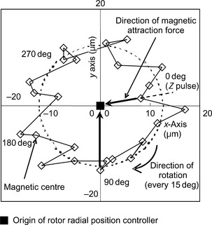
Figure 15.13 shows the waveforms of rotational speed ω, rotational speed command ω*, rotor displacements x and y, Z pulse, average torque command T*avg, and motor winding current command i*m, for a step change in speed reference from 1500 to 2500 r/min. It is seen that stable operation can be obtained at zero mean torque. However, the rotor shaft vibrates during the acceleration, i.e., during the high torque period. A magnetic attraction force (unbalanced magnetic pull) is always produced since the rotor is never at the stator centre as shown in Figure 15.12. The vibration of the rotor is higher during this period because the magnetic attraction force is in proportion to the square of airgap flux density, which is significantly increased during acceleration as can be observed by the increase in motor winding current.
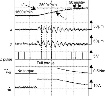
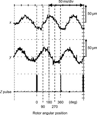
Figure 15.14 shows an enlargement of the waveforms during acceleration. The vibration of rotor shaft corresponds to the direction of magnetic attraction force caused by the circular movement of rotor centre. For example, at a rotor angular position of φ = 0 deg, the rotor radial position is situated along the negative x-direction from the stator centre and the magnetic attraction force acts in the same direction. As a result, the rotor is pulled further along the negative x-direction. Similarly, at a rotor angular position of φ = 90 deg, the rotor is pulled along the positive y-direction. This confirms that the magnetic attraction force caused by the circular movement of rotor centre is one cause of vibration.
15.6.2 A feed-forward compensator
In order to suppress the radial vibration it is necessary to compensate the magnetic attraction force by cancelling the magnetic forces caused by the circular movement of rotor centre around the stator centre. For that purpose, it is important to derive accurate theoretical formulae for the magnetic attraction force.
The locus of rotor radial position in Figure 15.12 is described by:
where xe and ye are the radial positions of the rotor in a two-axes reference frame and γe is the radius of the locus which was measured as 13 × 10−6 m. The magnetic attraction force due to phase A when considering the locus of the rotor position, as expressed in (15.28) and (15.29), can be written as
where, Fumx, Fumy, Fusx and Fusy are the magnetic attraction forces produced by ima, isa1 and isa2 in the x and y directions. Kum (θe) and Kus(θe) are coefficients of the magnetic attraction force where
and θe is the rotor angular position from the aligned position of the excited phase. The magnetic attraction forces for the B and C phases can be similarly derived. The magnetic attraction forces are proportional to the rotor displacements x and y and the square of stator winding currents. In addition, if rotor and stator poles are aligned, the magnetic attraction force is the maximum. As the rotor rotates from the aligned position, the magnetic attraction force becomes less (as previously stated).
Figure 15.15 shows the rotor radial position controller with the addition of a feed-forward compensator based on (15.30–15.33). (The feed-forward compensator is surrounded by the broken line.) If the locus of the rotor centre is not a circle, it is still possible to compensate the magnetic attraction force without a time delay by means of accurately measuring the locus.

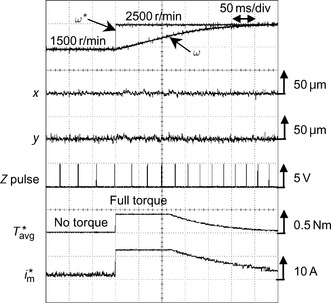
Figure 15.16 shows the experimental waveforms for a step change in speed reference with the feed-forward compensator. The conditions are the same as Figure 15.13. The operation of the motor is now stable in spite of the sudden step change. Therefore it is found that the feed-forward compensator is extremely effective in reducing the radial position variation caused by the circular movement of the unbalanced magnetic pull.
References
[1] Stephens, C.M., “Fault Detection and Management System for Fault Tolerant Switched Reluctance Motor Drives”. in Conf. Record of IEEE-IAS Annual Meeting, 1989:574–578.
[2] Ferreira, C.A., Jones, S.R., Heglund, W.S., Jones, W.D., “Detailed Design of a 30-kW Switched Reluctance Starter/Generator System for a Gas Turbine Engine Application”. IEEE Trans. on IA, Vol. 31, 1995:553–561. [May/June].
[3] Radun, A.V., Ferreira, C.A., Richter, E., “Two-Channel Switched Reluctance Starter/Generator Results”. IEEE Trans. on IA, Vol. 34, 1998:1026–1034. [September/October].
[4] Krishnan, R., Arumugan, R., Lindsay, J.F., “Design Procedure for Switched-Reluctance Motors”. IEEE Trans. on IA, Vol. 24, 1988:456–461. [May/June].
[5] Miller, T.J.E., “Faults and Unbalance Forces in the Switched Reluctance Machine”. IEEE Trans. on IA, Vol. 31, 1995:319–328. [March/April].
[6] Sawata, T., Kjaer, P.C., Cossar, C., Miller, T.J.E., Hayashi, Y., “Fault-Tolerant Operation of Single-Phase SR Generators”. IEEE Trans. on IA, Vol. 35, 1999:774–781. [July/August].
[7] Rahman, K.M., Fahimi, B., Suresh, G., Rajarathnam, A.V., Ehsani, M., “Advantages of Switched Reluctance Motor Applications to EV and HEV: Design and Control Issues”. in Conf. Record IEEE-IAS Annual Meeting, 1998:327–334.
[8] Shimada, K., Takemoto, M., Chiba, A., Fukao, T., “Radial Forces in Switched Reluctance Type Bearingless Motors” (in Japanese). in Proc. 9th Symp. Electromagnetics and Dynamics (The 9th SEAD), 1997:547–552.
[9] Takemoto, M., Shimada, K., Chiba, A., Fukao, T., “A Design and Characteristics of Switched Reluctance Type Bearingless Motors”. in Proc. 4th Int. Symp. Magnetic Suspension Technology, Vol. NASA/CP-1998-207654, 1998:49–63. May
[10] Takemoto, M., Chiba, A., Akagi, H., Fukao, T., “Radial Force and Torque of a Bearingless Switched Reluctance Motor Operating in a Region of Magnetic Saturation”. in Conf. Record IEEE-IAS Annual Meeting, 2002:35–42.
[11] Takemoto, M., Chiba, A., Fukao, T., “A Method of Determining the Advanced Angle of Square-Wave Currents in a Bearingless Switched Reluctance Motor”. IEEE Trans. on IA., Vol. 37, 2001:1702–1709. [November/December].
[12] Takemoto, M., Chiba, A., Fukao, T., “A New Control Method of Bearingless Switched Reluctance Motors using Square-Wave Currents”. in Proc. 2000 IEEE Power Engineering Society Winter Meeting, CD-ROM, 2000. [January].
[13] Takemoto, M., Chiba, A., Fukao, T., “A Feed-Forward Compensator for Vibration Reduction Considering Magnetic Attraction Force in Bearingless Switched Reluctance Motors”. in Proc. 7th Int. Symp. Magnetic Bearings, Zurich, Switzerland, 2000:395–400. [August].
[14] Takemoto, M., Suzuki, H., Chiba, A., Fukao, T., Rahman, M.A., “Improved Analysis of a Bearingless Switched Reluctance Motor”. IEEE Trans. on IA, Vol. 37, 2001:26–34. [January/February].