
Antennas
An antenna is a device designed to accept RF power from a transmitter and radiate it into its surroundings, or alternatively to extract energy from a passing radio wave and deliver it to a receiver. Considering transmitting first, an antenna is ideally designed to present a resistive load Rt = Rr + R1 (a pure resistance equal to the design load impedance of the transmitter, usually 50 Ω, if perfectly tuned and matched) and it is to this resistance that the transmitter delivers power. If the antenna is also loss-free, all the power delivered to it goes into the radiation resistance Rr and is radiated; if not, a proportion of it is converted into heat in the antenna’s loss resistance R1. The efficiency η of an antenna is given by η = ![]() . An ideal isotropic antenna is loss-free and radiates power in all directions with an equal intensity; it is a figment of the imagination as Maxwell’s equations describing electromagnetic radiation do not permit of such a design, but it is a useful yardstick for practical antennas.
. An ideal isotropic antenna is loss-free and radiates power in all directions with an equal intensity; it is a figment of the imagination as Maxwell’s equations describing electromagnetic radiation do not permit of such a design, but it is a useful yardstick for practical antennas.
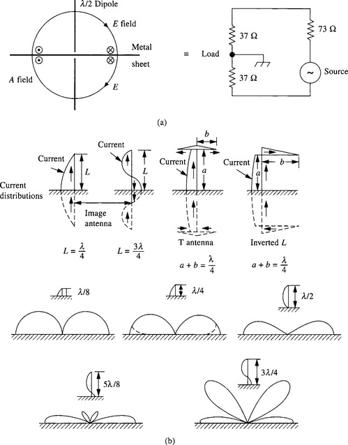
Practical antennas fall into two main groups, those which are self-resonant and those which are not. But note that in use, non-resonant antennas are often brought to resonance, e.g. with the aid of an ATU ‘antenna tuning unit’. The simplest resonant antenna is the half-wave dipole (known in the Americas as a doublet), the fields in the vicinity of which are shown in Figure 13.1. Figure 14.1a shows its figure-of-eight vertical radiation pattern in cross-section. The radiation intensity is a maximum in the plane at right angles to the dipole and is ‘doughnut’ shaped; there is no radiation along the line of the dipole. A vertical dipole is described as ‘vertically polarized’ since the lines of electric field in the direction of maximum radiation are vertical. As can be seen, the two halves of the figure eight are not quite circular. They are exactly circular for a dipole very much shorter than half a wavelength, but such an antenna is not resonant. In the direction of maximum radiation, the field strength produced by a lossless resonant ![]() dipole is 1.28 times that of an isotropic radiator, or ‘2.15 dB above isotropic’, whilst for a (suitably-matched loss-free) short dipole it is 1.22 times (1.76dB). When considering a perfectly-matched lossless dipole, these figures also represent the ‘directivity’ or gain relative to an ideal isotropic antenna. However, the term ‘gain’ should be restricted to the ratio of the actual maximum field produced by an antenna, relative to that which would be produced by an ideal isotropic antenna, i.e. ‘gain’ takes into account an antenna’s losses due to R1. Only in the case of a perfectly-matched lossless antenna does the directivity equal the gain in the maximum direction. In the case particularly of antennas which are not self-resonant, the difference between gain and directivity can sometimes be very large, even when the antenna is brought to resonance by tuning.
dipole is 1.28 times that of an isotropic radiator, or ‘2.15 dB above isotropic’, whilst for a (suitably-matched loss-free) short dipole it is 1.22 times (1.76dB). When considering a perfectly-matched lossless dipole, these figures also represent the ‘directivity’ or gain relative to an ideal isotropic antenna. However, the term ‘gain’ should be restricted to the ratio of the actual maximum field produced by an antenna, relative to that which would be produced by an ideal isotropic antenna, i.e. ‘gain’ takes into account an antenna’s losses due to R1. Only in the case of a perfectly-matched lossless antenna does the directivity equal the gain in the maximum direction. In the case particularly of antennas which are not self-resonant, the difference between gain and directivity can sometimes be very large, even when the antenna is brought to resonance by tuning.
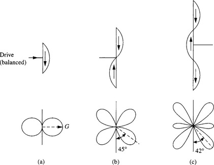
Figure 14.1 Current distributions on, and vertical radiation patterns of, vertical dipoles remote from the ground. The power gain G of an ideal lossless λ/2 dipole in horizontal plane is G = 1.65 (+2.15 dB) relative to isotropic
Due to end effects, a thin wire radiator such as that in Figure 14.1a has an electrical length which is about 0.025λ longer than its physical length. Like all resonant circuits, a resonant antenna has a bandwidth depending upon the circuit constants. For thin wire dipoles - length/diameter of the order 500:1 - the useful bandwidth for transmitting is about +/-10%, limited by the increase in VSWR away from the resonant frequency; rather more for receiving, where a worse VSWR is usually acceptable.
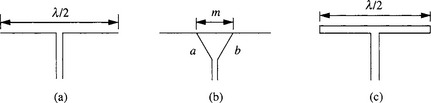
The bandwidth of a dipole can be increased by making the conductors very fat - tubes or wire cages - over most of their length, tapering conically to the feedpoint. A variant on this theme, the discone antenna, is illustrated in Figure 14.2. The operating frequency range may be increased if an ATU (antenna tuning unit) is used to bring the dipole back to resonance. The ATU actually decreases the ‘instantaneous bandwidth’, but the ATU can retune the dipole to resonance when a different operating frequency is required. For very broadband signals, the instantaneous bandwidth of an antenna can be increased by a technique known as compensation [1]. The impedance of a centre-fed λ/2 dipole (Figure 14.3a) is low and resistive, typically 73 Ω balanced. To generalize, it is low for dipoles an odd number of half-wavelengths long, and high for an even number of half-wavelengths (e.g. Figure 14.1c and b respectively) as is clear from the current distributions. For other lengths the impedance is not resistive; such dipoles are not resonant. The radiation patterns for dipoles having lengths of multiples of the half-wavelength at the operating frequency show additional lobes, e.g. for lengths 1 and 1.5 times the wavelength (see Figure 14.1). Note that the number of lobes is equal to twice the number of half-wavelengths. The patterns shown are for antennas in free space, i.e. remote from the ground, which would act as a reflector and modify the patterns.
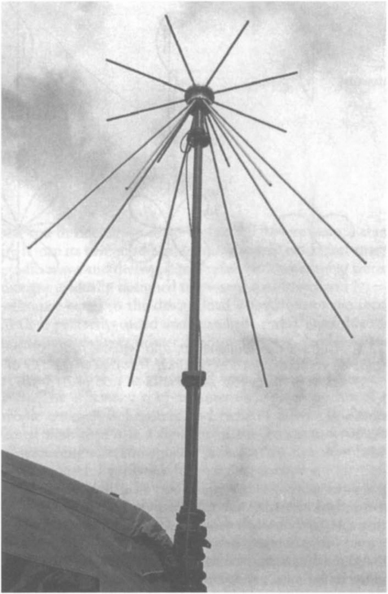
Figure 14.2 959 ‘helicone’ skeleton discone antenna, rated 30-76 MHz, 50 W. The elements are plastic-sheathed copper-plated steel helical springs so the antenna is small, light and virtually unbreakable. (Reproduced by courtesy of Racal Antennas Ltd., www.racalantennas.com)
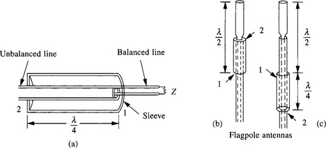
The 73 Ω impedance of the half-wave antenna of (Figure 14.3a is not convenient for connecting to a balanced twin wire feeder, which usually has an impedance of about 300 Ω, but this can be accommodated with a ‘delta match’ (Figure 14.3b). On the other hand, 75 Ω coaxial cable is about the right impedance for direct connection, but is unbalanced. A 1:1 ratio balun transformer (see Chapter 4) could be used, but this is a broadband device which is rather a waste as the dipole is inherently a narrow band radiator. A narrow band balun can be realized in various ways as in (Figure 14.4, and with proper choice of dimensions can also match the antenna to a 50 Ω cable, this impedance being preferred for transmitting systems. For receiving, e.g. for UHF Band IV/V TV, 75 Ω coax is commonly used without a balun, the balanced to unbalanced transition taking place gradually over a distance of several wavelengths along the feeder. Note that a wavelength in the cable is only about 0.6λ, as the velocity of the signal in the cable is only about 60% of that in free space. For VHF FM, a balanced 300 Ω twin wire feeder is often used and here the folded dipole of Figure 14.3c is useful. The two close-spaced dipoles act as a 2:1 turns ratio transformer, transforming the 73 Ω impedance of the simple λ/2 dipole to 292 O. A feeder which passes close to a source of interference is less prone to pick-up if it is balanced; in the case of an unbalanced feeder, an interference voltage may be induced in series with the outer, dividing (not necessarily equally) between the antenna and the receiver. In the case of a balanced feeder, the interfering voltage is induced equally in both conductors of the pair as a common-mode or ‘push-push’ signal, whereas the receiver (ideally) only responds to the normal mode (transverse or push-pull) voltage between the conductors. Incidentally, a folded dipole is often used in a Yagi multi-element antenna, connected to a 75 Ω feeder. The explanation is that one effect of the parasitic elements (reflector and directors) is to greatly reduce the impedance of a simple λ/2 dipole: using a folded dipole restores the desired 75 Ω impedance level.
The antennas which have been considered so far are balanced types. The operation of unbalanced antennas can be approached by looking at the performance of a modified balanced antenna. (Figure 14.5a shows a vertical λ/2 dipole with a horizontal metal sheet of very high conductivity and infinite in extent (a copper sheet extending many wavelengths would be an adequate approximation) inserted between the two halves, and its equivalent circuit. Note that the electric lines of force all meet the metal sheet at right angles and so are unaffected, whilst the circular horizontal magnetic lines, being parallel to it, do not cut the conductor and so are also unaffected. Therefore the field pattern is likewise unaffected, half the power being radiated above the plane and half below. If now the lower dipole element is removed and all the power fed into the top element (taking care to match the altered input impedance of 37 O), the far field of a λ/4 monopole above a conducting plane is seen to be the same shape as the upper half of the pattern for a λ/2 dipole but 3 dB higher in strength, or 5.15 dB above isotropic. The conducting plane is usually a ‘ground plane’, e.g. soil of very good conductivity. If the ground plane is not perfect (e.g. normal soil conditions) then the main lobe does not extend down to ground level. This is shown dotted in Figure 14.5b for the case of a λ/4 monopole (but applies equally to the other patterns), and the VSWR of the antenna will be high. The VSWR can be greatly improved with a set of buried radial conductors or a chicken-wire earth mat extending out to a radius equal to the antenna height, but for any significant improvement in the low angle radiation the mat would need to extend so much further that it is usually not economic so to do. Figure 13.5b shows the case of various monopoles including top loaded λ/4 monopoles (T and inverted L, useful to minimize antenna height when the wavelength is long), and the ![]() monopole. Monopoles up to λ/2 high have only the main lobe, which comes down to ground level; at
monopole. Monopoles up to λ/2 high have only the main lobe, which comes down to ground level; at ![]() λ small secondary lobes appear and at
λ small secondary lobes appear and at ![]() these are as large as the lower lobes. (Note that the descriptions T and inverted L are usually applied to antennas which are very much shorter than λ/4 and consequently not self-resonant even with the top loading, and must be brought into resonance by inductive loading. Medium and long wave broadcast antennas are of this type. Here, the top capacity loading is used to bring the effective height of the antenna closer to the physical height.)
these are as large as the lower lobes. (Note that the descriptions T and inverted L are usually applied to antennas which are very much shorter than λ/4 and consequently not self-resonant even with the top loading, and must be brought into resonance by inductive loading. Medium and long wave broadcast antennas are of this type. Here, the top capacity loading is used to bring the effective height of the antenna closer to the physical height.)
In the case of an antenna elevated above ground, the situation is more complicated, the radiation pattern in the vertical plane depending upon the pattern of the antenna itself, its height above the ground plane, its polarization, and the nature of the ground. Horizontally polarized waves suffer a phase reversal on reflection, exactly so and without loss if over a perfect ground plane. Thus there may be considered to be an ‘image’ antenna below ground, energized in antiphase. Since all points at ground level are equidistant from the antenna and its image, there is no net radiation at zero elevation. Vertically polarized waves are not phase reversed at angles above the ‘peudo-Brewster angle’, but are phase reversed below it. For perfect ground, this angle is zero, giving a maximum of radiation at zero elevation angle. But in practice, with normal or even ‘good’ ground, the peudo-Brewster angle is not zero, so that for rays at grazing incidence, there is phase reversal on reflection and hence a null at zero elevation.
In the case of either horizontally- or vertically-polarized antennas, the radiation pattern in elevation may exhibit one or more lobes, depending upon the antenna height above ground. The greater the height (in wavelengths) of the antenna above ground, the more lobes will appear. On the other hand, the horizontal plane or azimuth pattern depends upon that of the antenna itself, so for the vertical dipole it will be omnidirectional, and for the horizontal dipole basically figure-of-eight.
Many investigations of the radiation patterns of various antennas have been carried out, both in simulation and by actual measurements (e.g. by overflying by helicopter fitted with a measuring antenna). Given the many different types of antenna, varying mounting heights and allowing for the wide range of frequencies used for communications, the possible permutations are infinite. (Figure 14.6 shows a computer-simulated radiation pattern of a horizontal half-wave dipole for use at 14 MHz, mounted at a height of λ/2 (10.7 m) above varying types of ground. The plot shows the radiation pattern in elevation, for a bearing of zero degrees in azimuth, where the radiation is a maximum, i.e. at right-angles to the line of the dipole. It can be seen that the size and shape of the main lobe are little affected by the ground conditions, whereas these strongly affect the radiation in the vertical direction, for the following reason.
Given the stated mounting height, the downward radiation reaches the ground in antiphase. Upon reflection, it suffers a phase reversal, so that the reflected wave at ground level is in phase with the upward radiation at the antenna itself. But by the time the reflected wave arrives back at the antenna, it is again in antiphase with the upward radiation at that point and therefore tends to cancel it. If the terrain beneath the antenna is a very good reflector, the reflected wave is barely reduced in amplitude, and so the cancellation is almost complete. Over poor ground, some of the energy radiated downwards penetrates the ground and is absorbed, whilst what is reflected may suffer a phase ‘reversal’ which is not exactly 180°. Thus the reflected wave arriving back at the antenna is reduced and cancellation is incomplete, leaving appreciable net radiation in the vertical direction.
If the antenna height is raised, the null (or minimum) in the vertical direction splits into two, either side of the vertical. The angular spacing between them increases as the height is raised further, with further nulls successively appearing and splitting likewise.
At a higher frequency, e.g. 30 MHz, the vertical radiation pattern of a horizontal halfwave dipole mounted at the same height in terms of λ, namely λ/2, is very similar to that of Figure 14.6. But mounted at the same physical height as the antenna of Figure 14.6, namely 10.7 m or approximately one wavelength, there will be two distinct lobes either side of the vertical. There is a deep null between them at an elevation angle of about 45°, where the radiation is 8 dB or more below isotropic in the case of good ground (high conductivity and permittivity) - much more in the case of sea water. On the other hand, with poor soil the null is only some 5 dB below isotropic, clearly better if the only path open to a distant receiver involves a take-off angle of 45°. Thus ‘good’ soil is not necessarily an advantage. With a 30 MHz half-wave horizontal dipole mounted at a height of 2λ m there are four lobes either side of the vertical. The deepest of these, at an elevation angle of about 14°, is very deep regardless of soil type, being some 10 dB below isotropic, the higher nulls being progressively less deep, except in the case of sea water. In many cases, HF communications are typically required over paths of a given length; mainly short paths - for example tactical comms - or alternatively mainly medium to long paths, e.g. diplomatic traffic. Thus an antenna mounting height would be chosen to avoid a null at the required take-off angle over the usual range of operating frequencies.
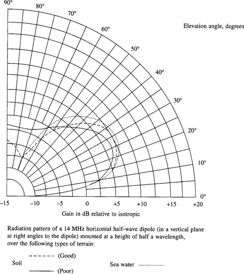
Figure 14.6 Radiation pattern in a vertical plane at right angles to a 14 MHz horizontal half-wave dipole, mounted at a height of λ/2 (10.7 m), over various types of terrain
An antenna is a reciprocal device, exhibiting the same polar pattern when receiving as when transmitting. However, when transmitting, the surrounding field is a spherically expanding wavefront centred on the antenna. As a receiver, the antenna experiences a passing plane wavefront, which excites an emf at the antenna’s terminals. For a λ/2 dipole, the emf is 2/p times lE, where l is the length of the dipole in metres and E is the field strength in volts per metre. The emf is in series with Rt, which thus appears as the antenna’s source resistance. If the λ/2 antenna is attached to a matched load, then in accordance with the maximum power theorem, half the antenna’s open circuit terminal emf will appear across the load and as much energy is dissipated internally in the source as in the load. Unlike a conventional signal source, however, the power dissipated in the antenna does not appear as heat (assuming R1 is small), but is reradiated by the antenna as a spherically expanding wave with both near- and far-field components. Thus in the immediate vicinity of the antenna, the resultant field is due to the combination of the original plane wave and the spherical reradiated wave.
The maximum amount of energy which a loss-free receiving antenna can deliver to a matched load is related to its ‘effective aperture’ A, an area at right angles to the direction of propagation of the signal. A lossless isotropic antenna has an effective aperture A = λ2/4p, thus A is a function of the wavelength and does not depend upon the physical size of the antenna. For practical antennas, A = Gλ2/4p, where G is the power gain of the antenna; thus a lossless dipole has an effective aperture A = 1.65λ2/4p.
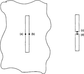
Babinet’s principle is an important consideration in some aspects of antenna design, notably broadband antennas. Babinet’s principle [5] relates the field solutions of complementary radiator configurations. Figure 14.8 shows a radiator consisting of a slot in an indefinitely large sheet of metal, energized by the application of a voltage between the points a and b. Also shown is an antenna consisting of a strip of metal of the same dimensions as the slot and energized between the points c and d on a narrow cut across the middle. Babinet’s principle states that denoting the feedpoint impedances by Zslot and Zstrip, then ZslotZstrip = 1/4Z2, where Z = ![]() , the impedance of the medium in which the antennas are immersed. This will usually be air (or space), when Z = 377 Ω the characteristic impedance of free space.
, the impedance of the medium in which the antennas are immersed. This will usually be air (or space), when Z = 377 Ω the characteristic impedance of free space.
A corollary is that if the metal areas of an antenna and the spaces between them are congruent, as in the spiral antenna of Figure 14.9, the antenna’s directivity gain, beamwidth and impedance remain constant over a broad frequency range, from one to many octaves, depending upon the particular design. This applies in two dimensions (e.g. a flat spiral like Figure 14.9 backed by a spaced off sheet metal reflector) and three (e.g. a conical log spiral antenna).

In many situations, from a VHF or UHF pocket pager to a military tactical HF communications system, size or weight considerations may enforce the use of an antenna that is much smaller than a half-wave dipole. Such an antenna will not be resonant in its own right, but measures can be taken to bring it to resonance. For example, a λ/4 dipole can be fitted with end discs, like the ends of a soft drinks can. Where the size is even smaller relative to a wavelength, either a loop or a dipole can be used and tuning components built in to bring it to resonance (Figure 14.10). However, with an electrically very small antenna, the radiation resistance becomes very low, with two important consequences. Firstly, as the ratio of the antenna’s reactance to R1 is high, when brought to resonance the Q will be high, giving a very narrow useable percentage bandwidth. Secondly, R1 will be much greater than Rr leading to a very low efficiency. Even if R1 could be reduced to zero (in principle one could use liquid helium and superconductivity to achieve this), the bandwidth would still be very narrow due to the high ratio of the reactance of the dipole or loop to the radiation resistance Rr. However, the aperture will be defined not by the physical size but by the wavelength, as noted above. Practical designs for passive electrically-small receiving antennas may well prove to have a gain G up to 20 dB or more below isotropic (though this does not necessarily apply to small active antennas). This low figure is entirely due to the loss resistance R1, a small dipole or loop will still have a directivity or gain-relative-to-isotropic. The literature covering electrically small antennas, which are mainly used for receiving, is extensive [5, 6].
At frequencies of 1 GHz and above, patch antennas can be useful. A patch or ‘microstrip antenna’ consists of a very thin flat metallic region or patch on a dielectric substrate, itself mounted on a ground plane larger than the patch; such antennas tend to exhibit a high Q value. If fed at two points with signals in quadrature, a patch antenna will produce circularly polarized radiation - or of course receive such radiation. However, if the patch is not quite square but slightly rectangular (often of a ‘perturbed’ design, i.e. one or more corners clipped) then the antenna will produce circularly polarized radiation with just a single offset feedpoint. But the bandwidth over which circular polarization results is smaller than that obtained with quadrature feeds and smaller even than that over which the VSWR is acceptable. However, such antennas are commonly used in GPS receivers. Depending upon the position of the feedpoint, the radiation produced will be either left-hand or right-hand circularly polarized; right-hand polarization is normally used. By their nature, patch antennas are unobtrusive, and can even be fitted to a curved surface, making them popular as aircraft antennas.
Circularly polarized radiation consists of two equal amplitude components of a wavefront travelling in the same direction. Relative to that direction, one component is vertically polarized and the other horizontally. If the two components were in phase, the result would simply be slant polarization at 45°. This could be received by a dipole at the appropriate angle, but would not be received if the dipole were turned through 90°. But with circular polarization, one component is in fact in phase quadrature with the other, and consequently the signal will be received, whatever the orientation of the dipole.
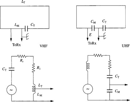
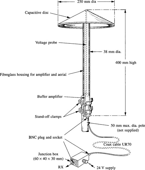
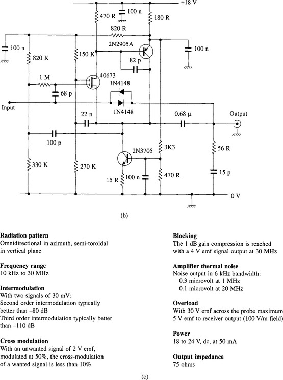
The foregoing relates to electrically small passive antennas. Where an electrically small antenna is intended for receiving only, an alternative approach to matching it directly to a feeder, is to design it as an active antenna. In the case of an electrically small dipole or monopole, the amplifier can be designed with a very high input impedance, or in the case of a small untuned loop antenna, with a very low input impedance, in each case the amplifier output being designed to match a standard feeder impedance, such as 50 O. Due to the small physical aperture of such an antenna, and the lack of matching, the signal energy available to the amplifier will be small, but provided it exceeds the amplifier’s internal noise by a sufficient margin, this will still allow satisfactory operation. In consequence, active antennas are particularly useful in the LF, MF and HF bands, where external noise greatly exceeds thermal noise, and is thus well above the internal noise of a suitably designed amplifier. Active antennas are offered by a number of manufacturers, in many cases the internal circuit design being a proprietary secret. Figure 14.11 shows an active HF antenna which, though no longer in the catalogue, is typical of the design of these antennas.
An active antenna such as that just described is effectively operated by the E field component of the signal. If an electrically small antenna must be situated in a position where it is subject to electrostatic interference, a loop antenna - which is operated principally by the H field of the signal - may prove more suitable. Figure 14.12, reproduced from Reference 8, shows such an active loop antenna, with gain switchable between about 8 dB or 20 dB. A three turn 15 inch diameter coil of 8AWG wire with ![]() inch turns spacing tuned with a dual gang 10-330pF capacitor covers 4.4 to 16 MHz. A single turn coil made by bending a 48 inch long strip of
inch turns spacing tuned with a dual gang 10-330pF capacitor covers 4.4 to 16 MHz. A single turn coil made by bending a 48 inch long strip of ![]() inch wide Ali sheet into a circle will cover from 13 MHz to beyond the top of the HF band, being useful at reduced performance right up to 55 MHz.
inch wide Ali sheet into a circle will cover from 13 MHz to beyond the top of the HF band, being useful at reduced performance right up to 55 MHz.

Figure 14.12 A high-frequency loop antenna. (Reprinted with permission from Electronic Design, July 22, 1996, Copyright 1966, Penton Publishing Co.)
Commercial loop antennas are available, offering very high rejections of electrostatic interference. These use a loop where the turn(s) are enclosed in an earthed screening tube.
A short gap in the tube prevents its presenting a shorted turn, enabling the H field to induce an emf in the inner, whilst screening the antenna from any electrostatic interference [8].
Transmitting antennas are usually required to have a higher efficiency than that which may be acceptable in a receiving system. Nevertheless, the laws of physics are immutable and one may have to accept an efficiency as low as a few per cent in the case of a tactical HF antenna at the lower end of the band. Such an antenna is ‘broadbanded’ by including load resistors which play no part at the higher frequencies where the antenna is not electrically small, but which keep the transmitter happy by maintaining the antenna’s VSWR within limits (e.g. less than 2.5:1) in the 2-4 MHz region where it is small in relation to λ. One such well-publicized antenna, popular with amateur radio operators, is shown in Figure 14.13: it is commonly known as the ‘Australian dipole’ and has also been tested and used by government agencies and commercial firms. With its overall length of 40.4 m, it is in fact only about 20% shorter than a half-wave dipole at its lowest rated frequency of 3 MHz, its main advantage being that it maintains a VSWR of 2.5:1 or better from there up to 30 MHz. But whilst presenting a reasonable match to a transmitter at all operating frequencies, ensuring that much of the available power is radiated, its actual radiation pattern is another question entirely. In azimuth it will be figure-of-eight, while the elevation pattern will depend upon the height at which it is mounted, and the frequency of operation. But in general, the elevation pattern will be multi-lobed at higher frequencies. It will be clear from the earlier discussion of antenna mounting height, that the actual antenna gain or loss relative to isotropic at any given elevation angle, at any frequency, will be somewhat uncertain, even varying with the degree of wetness of the ground in the vicinity.
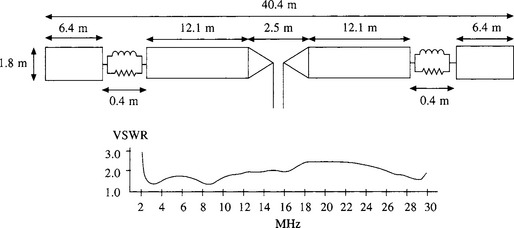
Figure 14.13 The ‘Australian dipole’ exhibits a VSWR of no worse than 2.5:1 over its operating range of 3 to 30 MHz
Another electrically small transmitting antenna which has created some interest in recent years is the ‘crossed field antenna’. It has been noted earlier that the E and H (electric and magnetic) fields in the vicinity of a dipole are in quadrature phase, so representing stored energy in what is effectively a tuned circuit, whereas radiation is only evidenced by the far field, where the E and H components are in phase, mutually orthogonal, and both orthogonal to the direction of propagation, as described by the Poynting vector. The crossed field antenna aims to synthesize the Poynting vector by producing separately stimulated E and H fields, and superposing them in the same ‘inter-action space’ around the antenna, to produce a radiated power flux S = ExH, where the x indicates a vector cross-product. The input power is split, and half applied to a pair of electrodes designed to produce the required E field pattern. The other half is used to produce a corresponding H field. One version of the system which has been described in the literature is said to cover 1.8-28 MHz, although it should be stressed that this is not the instantaneous bandwidth. The latter typically varies from about 100 kHz at 3.65 MHz to 400 kHz at 21 MHz, the elements of the splitter and phasing units requiring readjustment when the operating frequency is changed. The performance of the system is claimed to be good, but in view of its unorthodox approach this is disputed by many proponents of more conventional antennas.
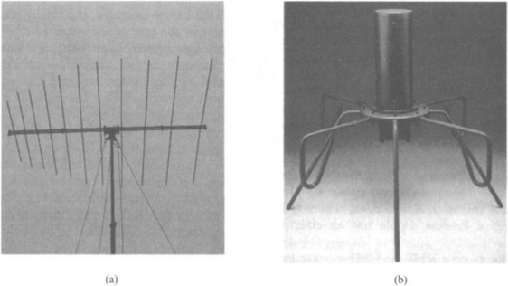
So far, only simple antennas, dipoles, monopoles, loops, etc., have been considered. Antennas with several elements can provide greater directivity than a dipole and thus exhibit an aperture (as far as transmission or reception in the preferred direction is concerned) of greater than 1.65λ2/4p. Antenna power gains G of up to 10 or 20 times (10-13 dB) are possible in HF antennas. Such high gain antennas are usually restricted to a fixed direction of operation, due to their size, but rotatable high gain HF antennas are available. (One type of antenna suitable for this purpose is the ‘log-periodic’ antenna, see Figure 14.7a, a multi-element antenna which can be designed to cover a relatively wide bandwidth.) This naturally presupposes one knows where the other end of the link is: for a more fluid situation, e.g. ground/air communications, or where messages must be broadcast to several vehicles, both ends of the link are likely to employ antennas designed to be as nearly omnidirectional as possible - no easy task on an aircraft. At VHF, gains in excess of 20 dB are possible, using array antennas such as stacked Yagis. (The Yagi antenna, which is narrow band, consists of a half-wave dipole plus parasitic elements which modify the pattern; a reflector behind the main element and a number of directors in front of it.)
(a)RA752VHF log periodic directional antenna, rated 30–88 MHz, 400 W. For lightness, economy and ease of transportation, the longer elements are loaded, allowing their physical length to be less than their electrical length
(b) RA978 UHF ground-to-air omnidirectional monopole antenna, rated 220–400 MHz, 1.2 kW pep. Available in both CAA and NATO codified versions
(Reproduced by courtesy of Racal Antennas Ltd., www.racalantennas.com)
For a thin wire half-wave dipole, the aperture of 1.65λ2/4p square metres seems to bear little resemblance to the actual area, which is clearly much less than this. However, with a large antenna array, or a dish antenna, where the overall dimensions may be many wavelengths, it is found that the actual physical area does approximate to the effective area A = Gλ2/4p. For example, a microwave dish of physical area a, will have an effective area of A = 0.6a, approximately. (The factor 0.6 is due to the impossibility of designing a feed system which will distribute the power uniformly over the reflector without spilling any over the edge.) Thus at microwave where dish antennas are commonly employed, gains of 40-50 dB are available.
In all cases of directional antennas, the increased gain in the desired direction is bought at the expense of reduced gain in other directions. With high gain antennas, there are usually a number of ‘sidelobes’, directions in which the gain, though much less than that in the main lobe, is nevertheless considerable. In some cases a directional antenna is employed more to discriminate against unwanted signals coming from a different direction from the wanted signal, than to increase the gain to the latter. A common example is in TV reception, where an antenna with a high front-to-back ratio can reduce ghosting due to reflections of the wanted signal, or interference due to another station. The examples just given are mostly terrestrial situations; only in space applications or in microwave links using very directional dish antennas will the free-space path loss formula be applicable.
So far, only individual antennas have been considered. The chapter would not be complete, however, without some mention of antenna arrays. These may be used for a number of purposes. For instance, an in-line array of antennas, all fed with equal amounts of power in the same phase from a transmitter via a splitter, will produce narrow beams, like a long thin figure-of-eight at right angles to the array, plus various sidelobes. On the other hand, if each individual antenna is fed with the signal, in equal amounts but suitably successively delayed in phase, a narrow end-fire beam is effected. Such linear arrays, given the necessary adjustable phasing arrangements, can be used as directional receiving antenna systems, and hence also as DF (direction finding) systems. Circular arrays of monopoles are used in DF systems at HF, such as in the Wullenweber system (where the large aperture permits the synthesis of narrow beams, especially in the upper part of the HF band) and at VHF, e.g. short range coastal DF installations. Compact arrays are necessary where space is limited, e.g. the Bellini-Tosi antenna (consisting of crossed triangular loops connected to a goniometer) once commonly used for ship-borne DF. Another example is the Adcock DF antenna (consisting of four vertical half-wave dipoles mounted at the ends elevated cross-arms and connected to phase-difference measuring equipment) for tactical DF applications, where rapid redeployment is a requirement.
A major accuracy limitation in DF systems, at both HF and VHF, is due to the reception of different rays, i.e. different versions of the same signal via different paths. At HF, these will usually be different skywave paths, whilst at VHF there may be both direct and reflected rays; both are examples of multipath propagation. In addition, in the tactical environment there is often great interest in DF on co-channel signals.
The simplest fixed two antenna array can give the bearing of an intercepted signal, but cannot distinguish between the true bearing and a ‘reciprocal’ bearing, at 180°. In some applications, e.g. in a tactical military environment, this will not be a problem, since enemy signals will originate from beyond the FLOT (front line of own troops). In other cases, the ambiguity can be resolved if the antenna array can be rotated slightly - if the array is moved anticlockwise, the phase of the signal in the right-hand element will advance relative to that in the left-hand element provided the signal source is in front of the array, or retard if behind. This the basis of some covert vehicle-borne tracking systems.
If the array is receiving one unique signal, via a single path, the amplitude of the signals from the two antennas will be equal, at least when the target is dead ahead. If they differ, this indicates that the signal is comprised of two ‘rays’ or wavefronts, arriving from slightly different directions. On the basis of an assumption that both arrive at the same low elevation angle, likely at VHF but unlikely at HF, it may be possible to estimate the two rays, but in many cases, e.g. with HF signals or more than two rays, this will be impossible. If an additional antenna or two is added to the array, much more data become available, and the process has been carried further.
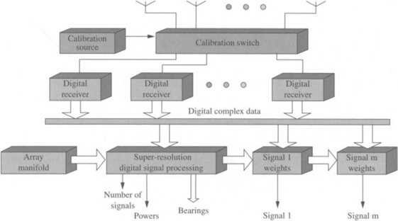
Figure 14.14 is the block diagram of the hardware developed to run advanced SRDF (super-resolution direction finding) algorithms such as MUSIC (multiple signal classification) on signals gathered from an eight antenna array. The system copes with multi-path reception of signals and with multiple signals on the same channel. The SRDF algorithms require knowledge of the antenna array layout, i.e. the relative x, y and z (height) co-ordinates of the individual antennas, some irregularity in the layout being positively beneficial. Using SRDF, small tactical arrays can provide similar performance to that previously only achieved with much larger fixed site arrays [9]. The system also provides an adaptive beam-forming capability. This permits a beam to be formed in the direction of an intercepted signal of interest, whilst simultaneously steering nulls in the direction of all other signals, subject to there not being too many relative to the number of antennas in the array.
Many member states of the ITU maintain monitoring stations, to help police the usage of frequency allocations etc. The UK Radio Agency’s monitoring station at Baldock now uses an SRDF system, making use of a subset of antennas in a pre-existing large HF receiving array, and similar systems are in use in North America, Australia and various European countries.
SRDF systems can also provide good results in difficult installations, such as on board warships. Here, the most favoured antenna position, at the top of the highest mast, is generally not available to a DF installation, and all other antenna locations naturally suffer severe local multi-path, due to reflections from the ship’s superstructure. Special techniques, including calibration against known targets over the full range of bearings in azimuth, enable SRDF algorithms to work under these extreme conditions.
Finally, there are specialized antennas for field-strength measurements. These are covered in Chapter 16, Measurements.
References
1. Kraus. Antennas, New York, McGraw-Hill, 1950.
2. Jasic. Antenna Engineering Handbook. McGraw-Hill: New York, 1961.
3. Schelkunoff, Friis. Antennas, Theory and Practice, New York, John Wiley and Sons, 1952.
4. Terman. Radio Engineering, 3rd edn, McGraw-Hill, New York, p. 716
5. Antenna Handbook Y. T. Lo, S. W. Lee (Eds) Van Nostrand Reinhold Co. (With excellent index)
6. Sept–Dec, Virani. Electrically small antennas. Journal I.E.R.E., 1988;538(6):266–274.
7. Fujimoto et al. Small Antennas, Research Studies Press
8. Salvati. High-Frequency Loop Antenna. Electronic Design, 1996;22, July
9. Tarran. HF tactical superresolution DF and adaptive beamforming