Propagation

This chapter and the succeeding one between them cover the topics of antennas and propagation. These topics are closely interlinked. Both are very wide ranging subjects, so it will only be possible to scratch the surface in these two chapters. There is a vast quantity of literature relating to each of these topics, and from it, a small selection of references has been included at the end of each chapter, for further reading. In addition to propagation, the topic of external noise (both naturally occurring and man-made) is, for convenience, also covered in this chapter since (together with antenna gains and propagation loss), it determines the transmitter power needed to communicate over any given path.

The topics of antennas and propagation are closely interrelated, so it will be helpful to start a consideration of propagation with a look at the electric and magnetic field distributions both close to and far from a basic dipole antenna, although the main treatment of this antenna is reserved for Chapter 14. Figure 13.1 shows the electric and magnetic fields from a vertically polarized dipole radiator. The electric field is everywhere at right angles to the magnetic field and both are everywhere at right angles to the direction of radiation. (This condition can be met in two dimensions but not in three, which is why an isotropic radiator is not possible. An isotropic radiator would radiate an equal intensity signal - or alternatively receive equally well - in all directions. Although not physically realizable, it is a useful yardstick for comparing other antennas.) The electric lines must start and finish on the conducting elements of the dipole, whilst the magnetic lines must form closed loops encircling the current flowing in those conducting elements. The current flowing in the elements of a resonant λ/2 dipole is (almost) in quadrature with the applied voltage, so the electric and magnetic fields in space close to the dipole are also in quadrature; this is the ‘near field’ region. The associated energy circulates back and forth between the electric and magnetic fields, exactly as in a tuned circuit and the Q value of the antenna determines its 3 dB bandwidth in exactly the same way as for a tuned circuit. When exactly on tune the antenna looks resistive to the source since the latter only supplies the energy ‘consumed’ by the radiation resistance R_r (and by the loss resistance R₁, although in a well designed efficient antenna, this may amount to as little as a few per cent of the power radiated). The quadrature electric and magnetic fields close to the dipole are called ‘induction fields’ and they drop off more rapidly with increasing distance from the dipole than do the electric and magnetic components of the radiation field. The latter are in phase with each other and thus describe a flow of power radiating outwards from the antenna.

Beyond a few wavelengths from the antenna, the radiation field greatly exceeds the induction field; this is called the far field region, where the radiated energy expands as a spherical wavefront centred on the radiator. (At a great distance from the antenna, the radius of this spherical wavefront becomes so great, that to a receiving antenna, it appears as a plane wavefront.) The magnetic field is associated with current and the electric field with voltage and their ratio is a resistance. This is called the characteristic resistance of free space, and has the value 120π or 377Ω Consider the power W watts flowing through a small area A (in units of square metres) on the surface of such a sphere (Figure 13.1): then the field strength η in volts per metre is given by η = √(377Φ), where Φ is the power density W/A. For each doubling of the distance from the radiator, the power is spread over four times the area. Thus the power available to a receiving antenna falls to one-quarter for a doubling of the distance, giving the attenuation of a radio wave in a lossless medium (free space) as an inverse square law or − 6 dB per octave (doubling) of distance. In a radar system, such energy as is scattered by a small target back in the direction of the radar set is also subject to the inverse square law, giving the basic radar range law as R⁻⁴ or inverse fourth power of range. Where the target fills the field of view of the antenna in one dimension (e.g. the horizon) or two dimensions (large cloud bank), the range law becomes R⁻³ or R⁻² respectively. By contrast, metal detectors work upon the more rapidly decaying induction field (near field) and so are subject to an R⁻⁶ range law.

Turning now to a complete radio communication path, the path loss between isotropic antennas in free space, defined as the ratio of transmitted power P_t to received power P_r is (4πd/λ)2, assuming d (distance) is large compared with λ, d and λ both in metres. For two half-wave dipoles (broadside on to each other), the loss will be less, since each has a gain in the maximum direction of 2.15dB (×1.65) relative to isotropic, giving P_t/P_r = (2.44πd/λ)²; so for example at a spacing of 10λ, the received power is 1/5876 times the transmitted power. Due to the × 6 dB/octave (inverse square) law, the received power will be four times as great every time d is halved. On this basis, when the separation is 1/(2.44π) times a wavelength, there is no loss at all between a pair of half-wave dipoles, and at half this separation the received power is four times as great as the transmitted power! Of course, the formula only holds for the far-field region, not for a spacing as small as λ/(2.44π) = 0.13λ. Nevertheless, using 0.13λ as a starting point, with a little practice at the mental arithmetic you can astound your colleagues by working out the free-space path loss for a communications system in your head. For example, at 144 MHz λ is approximately 2 m and at a separation of 0.25 km (approx. 1000 times 0.13λ or 2¹⁰ times or 10 octaves of distance), the free-space loss between half-wave dipoles is simply (10 × 6) = 60 dB. An alternative starting point that can be useful to memorize, is that the path loss between isotropic antennas separated by a distance equal to λ, is 22 dB.

Where the antennas have a different value of gain, this must be allowed for, leading to the formula

where G_tG_r is the power gain relative to isotropic of the transmit, receive antenna in the required direction respectively.

The above formula may be re-expressed to give the free-space path loss L in decibels as follows

L = (32.44 + 20 log₁₀f+ 20 log₁₀d) dB, for the case of isotropic antennas (G_t = G_r = unity), or

L = (28.15 + 20 log₁₀f+ 20 log₁₀d) dB, for the case of isotropic antennas (G_t = G_r = ×1.65), or where frequency f is in MHz and distance d is in km.

In many cases we need to know the path loss taking into account the effect of the surrounding terrain. The following deals only with paths short enough to be considered as over flat earth; there are formulae for the curved earth case, but for paths long enough for the effect of the earth’s curvature to be important, the range is generally determined by factors other than those considered below. The following also refers to cases where the ground wave can be neglected, namely higher frequencies: ground wave propagation is dealt with in a later section.

Figure 13.2a shows antennas that are vertically polarized, but the following applies also to horizontally polarized antennas. The voltage induced in the receiving antenna is the resultant obtained by adding the direct and the reflected rays. If the angle θ at which the incident ray strikes the ground is very small, then the reflected ray will suffer a phase reversal. In the case of smooth ground (or calm water), the reflected ray is little attenuated (even if the ground is of poor conductivity) and so its magnitude at the receiving antenna will be nearly the same as the direct ray. If the difference in the lengths of the paths taken by the direct and indirect rays is small compared with the signal’s wavelength λ, then the two versions of the received signal will be nearly in antiphase. Under these conditions, the received signal amplitude will be directly proportional to the phase shift between the two rays, Figure 13.2b. The received signal level will therefore be considerably less than it would be if the direct ray were received in the absence of the reflected ray. From the geometry of the situation and taking account of both the free-space loss and the additional loss due to cancellation, the ratio of received to transmitted power P_r/P_t between isotropic antennas mounted at heights h_t and h_r separated by distance d is equal to (h_th_r/d²)², independent of units, provided both height and distance are in the same units, e.g. metres.

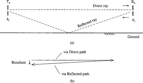
Note that unlike the free-space loss, this does not increase with frequency since as λ gets shorter, the phase shift between the direct and incident rays increases and hence so does the resultant. Note also that if the range is doubled, the antenna heights remaining unchanged, then due to the geometry (the angle between the direct and the reflected ray being halved) the angle between the vectors representing the direct and reflected rays in Figure 13.2b will also be halved. Thus the size of the resultant relative to the direct ray will be halved. But the direct (and reflected) ray is itself halved in amplitude, due to the doubled range. Thus the path loss is now proportional to the fourth power of d, i.e. the range law is now − 12 dB/octave of distance. Be careful when using this formula; remember it only applies if the phase shift between incident and reflected rays at the receive antenna is small. Always work out the free-space loss as well and distrust the original answer if it is not much greater than the free-space loss.

Both the free space and flat earth formulae above assume straight ray (LOS - line-of-sight) propagation. This is not always the case. Where a LOS path does not exist, communication may still be possible. In this case, the signal reaches the receiver by diffraction, or by penetration (more effective at lower frequencies), or by reflection (more effective at higher frequencies). For communication to be successful, the additional losses must be allowed for. These can be calculated for simple cases, or use may be made of measured values published in the literature. A great deal of work has been done on propagation at VHF and UHF in connection with PMR (private mobile radio) and mobile telephones, e.g. [1]. In this case, the base station antenna is elevated, but the mobile’s antenna is not, and will frequently be screened. A well known study was carried out by Egli (one of the earlier workers in the field) [2]. From a study of a large number of measurements made in large towns, he suggests that at frequencies above 40 MHz, an additional empirically-derived term (40/f)² (f in MHz) be inserted in the above equation. This is a median allowance for base-to-vehicle and vehicle-to-base paths: he also gives statistical spreads, which differ for the two cases. Figure 13.3 shows the predicted path loss versus range for communications in the region of 140 MHz.

The flat earth propagation formula, together with empirical adjustments suggested by Egli, Okamura and others, gives good guidance to the maximum range which can be expected for a given transmitted power at VHF and above, at least out to the ‘radio horizon’. The factors determining the distance of the radio horizon are complex, including antenna heights among other things. But briefly, the radio horizon is the distance beyond which the received signal strength falls off very rapidly. So rapidly in fact, that there is an upper limit to the transmitter power that it is worth using with a given antenna height. However, VHF/UHF signals may occasionally be received at distances well beyond the radio horizon, due to conditions such as a temperature inversion, ducting, etc., the effects often being evident as, for example, patterning on a TV set.

At HF and lower frequencies (30 MHz downwards) the same formulae still indeed apply, but the actual range is often found to far exceed that thus predicted for various reasons. Firstly, at lower frequencies, radiated power travelling parallel to the earth is slowed down at the earth/air interface due to the conductivity and the high dielectric constant of soil or water. As a result, the wavefront instead of being vertical, tends to tilt forward at higher levels and thus to follow round the curvature of the earth: this is known as the ground wave. Note that the ground wave is always vertically polarized; the conductivity of the earth short circuits any horizontally polarized component of the wave, eliminating any horizontal component of electric flux. At low frequencies the ground wave range is very extensive, so that for instance the BBC’s Droitwich transmitter (whose 198 kHz carrier frequency is maintained to an accuracy of 1 part in 10¹¹) can be received over much of continental Europe.

At even lower frequencies such as VLF (very low frequencies, 3-30 kHz) the ground wave extends for thousands of kilometres (an earth-ionospheric waveguide duct mode is also relevant here) and even penetrates the surface of the ocean very slightly, so that VLF can be used for world-wide communication with submarines, albeit at a very restricted data rate. At HF, the ground wave falls off much sooner: nevertheless long distance communication is still often possible. This is because ionized layers of the atmosphere (the ‘ionosphere’) reflect back towards the earth signals that would otherwise be lost into space (Figure 13.4). The signal, on striking the earth, is reflected and may then be reflected from the ionosphere a second time, to return to earth even further away. The distance from the transmitter to where the first reflection strikes the earth is known as the ‘skip distance’ and the area of no reception beyond ground wave range to where the first reflected signal is heard is known as the ‘dead zone’.

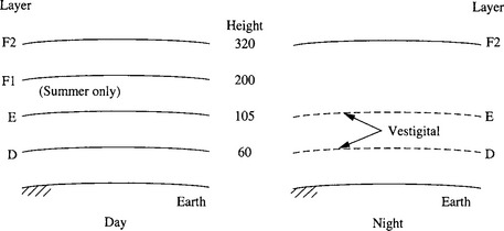
During the daytime, typically there are four ionized layers at different heights. The lowest, the D layer, is responsible for heavy attenuation at MW frequencies, giving interference-free reception of MW broadcast stations within their ground wave range during the hours of daylight. After dark, it almost disappears as in the absence of sunlight, the ions and electrons recombine; distant MW stations can then be heard via ionospheric reflections at ranges way beyond their intended primary ground wave service area, leading to severe interference with local stations. The attenuation of the D layer falls off at higher frequencies, which can thus penetrate it even during the hours of daylight. These frequencies are reflected from the E layer or one of the F layers, depending upon the time of day, the season and the current level of the sun’s activity, which exhibits short-term variations (over days) and long-term variations over the 11-year sunspot cycle.

For an HF communications link there will be at any given time an LUF (lowest usable frequency) set by the higher levels of absorption and of atmospheric noise prevailing at lower frequencies, and other factors such as E-layer cut-off, and an MUF (maximum usable frequency) beyond which the transmitted signal penetrates all the layers and does not return to earth. The strongest return occurs at just below the MUF, but it is better to work at a slightly lower frequency to allow for slight short-term variations in the MUF. Typically, communication is carried out at a frequency of about 85% of the monthly median of the F2 MUF; this is known as the OWF (optimum working frequency) or the FOT (frequence optimum de transmission) and is assumed to give a path for about 90% of the time, assuming communication is possible. For it can happen occasionally that the frequency range between the LUF and the MUF becomes vanishingly small. Though not a common occurrence, this is most likely to occur on long paths where part of the path is in daylight and part in darkness, or in trans-polar paths where high levels of absorption may raise the LUF until it equals or exceeds the MUF.

Choice of operating frequency may be left to the judgement of an experienced operator, choosing from among a limited number of assigned frequencies. However, experienced operators are becoming rare whilst the demand is for ever more reliable HF communications. To this end, computer programs are available to assist in calculating the best operating frequency for any given route at any given time; this might be for example a three-hop path via the E layer (3E) and/or a one-hop path via the F2 layer (1F2). Examples of such programs are APPLAB 4, from the Rutherford Appleton Laboratory, Didcot, Oxfordshire, UK, and ‘Muffy’. The latter program, though less sophisticated, can be run on a PC or compatible personal computer and is thus popular with amateurs.

Typically, a prediction program will give the required transmitted power for any paths that are ‘open’, taking into account the latitude and longitude of the transmitter and of the receiver and their heights above sea level, the receiver bandwidth, the type of antenna, the time of day, season, and sunspot number. Propagation prediction programs can only take into account known average conditions; they are unaware of any incidental short-term variations from these mean conditions. In particular, it would be wrong to think of the various ionized layers as perfect spherical mirrors encompassing the globe. In places they may exhibit dents, corrugations or other irregularities. These are transitory disturbances due to wind shear and other meteorological effects, with the result that a path between a transmitter and a receiver, predicted as open at a certain frequency by a program such as Applab, may in fact not be available to pass traffic, whilst a path not predicted as open may well provide an excellent signal at the receiver. There are also other more catastrophic effects, all associated with solar flares, traditionally considered unforecastable though hopefully progress is being made in this direction. These effects include:

It will be apparent from the foregoing that a certain amount of uncertainty exists as to whether communication is possible over a given path on one of the assigned frequencies available to the would-be communicator. Consequently, use may be made of another advanced aid to HF communications reliability, namely the chirp sounder. Various stations around the world transmit at different times at precisely known intervals a CW transmission which sweeps steadily across the whole HF band. A special purpose chirp receiver can receive the signal from the chirp sounding transmitter, displaying received signal strength and time delay of the signal versus frequency. The former enables a frequency offering an adequate signal to noise ratio to be chosen whilst the latter permits the avoidance of frequencies at which two or more paths are open. This is particularly beneficial for radio-telex or data transmissions, to minimize errors due to ISI (intersymbol interference). The time delay difference between paths is typically 2–3 ms with a normal maximum of 5 ms and a worst case of about 10 ms. Interestingly, the largest spread of delays is in fact experienced over short paths.

Where a special purpose chirp receiver is not available, use can still be made of chirp transmissions. It is only necessary to listen out on the intended frequency of communication (or an adjacent clear channel) for a chirp transmission from a transmitter near to the other end of the intended link. A characteristic up-chirp will be heard (or a down-chirp if using lower sideband) as the transmission sweeps through the receiver channel. Knowing the expected time of the sweep passing through the tuned frequency, and given an accurate clock, reception of the chirp will indicate that the path is open. By listening on other frequencies, the current values of the LUF and MUF, for the given path, can be estimated. Chirp-sounding transmitters are operated at various sites in the UK by various branches of the services, and by certain other agencies throughout the world at sites ranging from Oslo (NATO), Belize, Norfolk Virginia, the Philippines, Hong Kong, Canada, Saudi Arabia (with no less than three transmitter sites) and others. All stations transmit at the same sweep rate of 10 seconds per MHz, thus taking 4 minutes 40 seconds to cover the band 2-30 MHz. Some stations transmit a chirp every 15 minutes, others every 5 minutes. Each station has a unique start delay of so many minutes and seconds past the hour (or past the quarter hour, etc.), so that knowing this, and given the 10s/MHz sweep rate, the exact expected chirp time for any given transmitter can be determined for any particular receive frequency. Thus, given an accurate watch, any chirp received indicates an open path to the general location of the corresponding chirp transmitter.

The three ionospheric effects listed above and other variations also have an effect upon DF (direction finding) systems. SITs (systematic ionospheric electron density tilts) may result in an HF signal returning to earth at a different point from where it would have appeared had the ionosphere been smooth and regular. This can introduce an error in the measured bearing of the transmitter at one or both receiving stations of a DF system, resulting in the position indicated by the intersection of the cross bearings being inaccurate. SITs [3] have a particularly serious effect on single stations DF systems, which rely on measurement of the azimuth and elevation arrival angles, and an estimate of the height of the appropriate reflecting layer, to calculate both the bearing and distance of the target transmitter. Similarly, TIDs (travelling ionospheric disturbances) [4] produce gradients in the electron density, again resulting in propagation of an HF signal over a path which deviates from a great-circle direction.

Transmissions at frequencies above about 28 MHz normally pass through all the layers and do not return to earth. However, they may still be used for over-the-horizon communications in certain circumstances. A troposcatter link operates at microwave, depending upon irregularities in the troposphere to scatter a highly directional beam of microwave energy transmitted at a low elevation angle. Sufficient energy is directed back down again in a forward direction to permit reception at distances well beyond the horizon. There is also ionospheric scatter, which depends upon irregularities in the D layer. Meteorscatter communications use frequencies in the range 35-75 MHz. Here, communication is by reflection from the trail of ionized air left by the passage of a meteorite. This acts as a ‘wire in the sky’, capable of reflecting the incident energy to the receiving end of the link, if the polarization and orientation are right. The transmitting station repeatedly sends a short ‘message-waiting’ transmission, and on receiving a reply from the intended recipient, sends text, a packet of data or other message as required. The geometry of the path is critical, so that it is unlikely that the signal can be intercepted by other than the intended receiving station. As with troposcatter, for a fixed link, directional antennas can be employed with advantage. The abundance of meteor trails depends upon the time of day, season and latitude, so the waiting time for a path to occur may be anything from a few seconds to many minutes. The length of time for which a trail persists is anything from a few tens of milliseconds to a few seconds and during this time it offers a high integrity path capable of supporting a data rate of up to 10 kb/s or more. The unpredictable waiting time makes meteorscatter unsuitable for real-time traffic, but it is ideal for store-and-forward message operation.

A wealth of information on radio-wave propagation, both normal and anomalous, is available from many sources on the World Wide Web. For example, a variety of reports is available from Reference 5, while a Google search on ‘VHF Propagation’ or ‘UHF Propagation’ will produce numerous ‘hits’. These will explain that various effects are responsible for the occurrence of anomalous propagation paths at VHF and UHF, one important type being ‘inversions’, in some types of which fog or moist air plays a crucial role. Another type of inversion ‘abduction’, which is common in summer near large bodies of water, when hot dry air over land is blown across the water, and - under other circumstances - also in winter. It can result in the reception of distant UHF TV stations that are normally not receivable, and result in co-channel interference. Other types of inversion are ‘subsidence’, ‘nocturnal’ and ‘frontal’. Inversions may also occur at high altitudes, up to 1500 m or more, and two or more inversions may be stacked one above the other at different altitudes. This can result in ‘ducting’, in which a signal propagates as though it were in a waveguide rather than in free space, consequently travelling large distances without the attenuation attendant upon the free-space 1/R² range law.

The properties and uses of microwaves are so important and interesting that, although they lie beyond the frequency range with which this book is primarily concerned, a few words here will not come amiss. Propagation at microwave frequencies extends little beyond the optical horizon and in a well designed and set-up link the line of site path loss is often little greater than that predicted by the free-space formula. The 20 log₁₀f term in the free-space path loss formula might seem to suggest that very large powers would be needed to permit communication at microwave frequencies.

This would indeed be so if half-wave dipoles were used, as the effective aperture (see the next Chapter) of a microwave dipole is very small. However, due precisely to the short wavelength, it becomes possible at microwave frequencies to use dish antennas of diameter much larger than a wavelength (with a corresponding greatly increased aperture) at both the transmit and the receive ends of the link. Thus the term G_tG_r may well be much greater than 40 dB. Such dishes achieve their greatly increased effective aperture at the expense of omni-directional response and may have a beam-width of only a few degrees.

Any large city is criss-crossed by numerous microwave fixed communication links, mounted on the tops of high buildings. In these links, unlike a mobile scenario, the narrow beam-width is no disadvantage, in fact the very opposite, so that frequencies can be re-used in close proximity without danger of mutual interference. Due to their high gain antennas, such links commonly work with a transmitted power of just a few watts, often generated by a Gunn Diode transmitter.

On longer distance microwave links, say between stations mounted on hilltops or mountains, phenomena such as temperature inversions or ducting can sporadically interfere with transmissions, as happens with lower frequency transmissions. Other causes of temporary loss of communication include exceptionally heavy rain, especially at higher microwave frequencies where the dimensions of a raindrop are not negligible compared to the wavelength. Rain fades are usually not a problem in a well designed microwave link, however, as it will have been engineered to provide a 30 dB or so capability above and beyond the normal path loss. Where a direct line of sight path cannot be found, a link can often be engineered with the aid of a flat reflector, mounted atop a hill or tall building.

A clear line-of-sight path is the norm for one type of microwave link - satellite up- or down-links, the latter widely used for television transmissions. For this purpose, the satellite is maintained in a geostationary position, just under 36 km above a point on the equator.

In such a position a satellite TV transmitter can cover about a third of the globe, so three or four such satellites could cover the whole surface of the earth, with the exception of extreme northerly and southerly latitudes.

Geostationary satellites with highly directional antennas are also used for fixed links, providing carriers for thousands of intercontinental telephone channels. Another well-known application of geostationary satellites is the US Department of Defence Satellite Navigation System, commonly known as GPS (Global Positioning System) later joined by Glonass, operated by the Russian Federation, and possibly shortly by Galileo, a proposed European global positioning system. These systems each employ a ‘constellation’ of satellites, GPS and Glonass between them maintaining almost 50 satellites.

In any radio communications link, noise at the receiver sets the lower limit of signal strength which provides a usable signal. A received SNR (signal to noise ratio) of about +10 dB is required for speech and a similar figure suffices for fairly robust forms of digital modulation. The most robust types can operate with a signal to noise ratio of 0 dB or even a small negative SNR, as can a good CW morse operator, whereas very bandwidth-economical methods of modulation such as 64QAM or 256QAM (carrying 6 bits or 8 bits per symbol respectively) require a signal to noise ratio in excess of 20 dB. By contrast, a ‘direct sequence’ spread spectrum system (where the actual data rate is much lower than the modulation or ‘chipping’ rate), can provide up to 25 dB or more of processing gain’, permitting such a system to operate with a large negative signal to noise ratio.

The noise at the receiver comes from several sources. The first is the receiver’s own noise (internal noise), mainly attributable to the first active stage such as RF stage or first mixer; this noise is considered in earlier chapters. The noise with which we are concerned here is external noise and this arises from three sources. Atmospheric noise is mainly due to electrical storms in the tropical regions of the world, although other sources such as the aurora borealis (Northern Lights) and the aurora australis also contribute. The intensity of atmospheric noise varies with the time of day, season and the 11-year sunspot cycle, and also the geographical location of the receiver.

The second type of noise is galactic noise, which is of cosmic origin. This is largely invariant in intensity which is greatest in the direction of the galactic centre; it is only of importance in the frequency range 3–300 MHz, and then only at times and seasons of low atmospheric noise, and at sites where man-made noise is low.

The third and in many cases the most important type of noise is man-made noise. This arises unintentionally from a wide variety of sources and is either impulsive, e.g. from electric motors, vehicle ignition systems, light switches, thermostats, etc., or continuous such as radiation of clock frequency harmonics from computers, radiation from ISM (industrial, scientific and medical) RF generators used for diathermy, metal treatments, polythene sealing, etc. Man-made noise does not include disruption of radio reception by other radio transmissions (interference) - although in practice this may often be the major problem - or by deliberate attempts to prevent communication (jamming).

The levels of atmospheric noise experienced at various locations throughout the world at various times of day, season and phase of the sunspot cycle are comprehensively listed in Reference 6. Atmospheric noise usually predominates at frequencies up to 30 MHz and the report consequently concentrates on this frequency range. It should be noted that when a directional HF antenna located in temperate latitudes is used, the level of atmospheric noise encountered will be greater if the main lobe points towards the tropics than if it points towards the pole. At frequencies in excess of 100 MHz a receiver is likely to be internally noise limited. (However, note that at any frequency, an inefficient antenna, antenna feeder loss and the insertion loss of any filters ahead of the first stage of amplification will all attenuate both the wanted signal and the external noise, possibly leading to the receiving system being internally noise limited.) At microwave frequencies the external noise level is so low that (unless the antenna is pointed at a noise source, e.g. the sun) for very weak signals it is useful to take steps to reduce the receiver’s noise figure below the thermal noise level prevailing at room temperature. This may be done either by refrigerating the RF amplifier in liquid nitrogen or liquid helium, or by using a parametric amplifier. When designing a receiver it is useful to have guidance as to the minimum likely level of external noise, since there is no point in incurring additional cost to secure a receiver internal noise level much lower than this. Reference 7 gives this information for frequencies from 0.1 Hz to 100 GHz, covering atmospheric, galactic and man-made noise. For much of this frequency range it also gives some useful guidance as to the likely maximum levels. Figures 2 and 3 from this report are reproduced in this volume, by permission of the ITU-R, as Appendix 12. Between them, they more than cover all the frequencies used for radio communication with which this book is concerned, i.e. principally from 100 kHz to 1000 MHz.

References

1. 4 February, Ibrahim, Parsons. Urban mobile radio propagation at 900 MHz. Electronics Letters, 1982;18(3):113–115.
2. October, Egli. Radio propagation above 40MC over irregular terrain. Proceedings of the I.R.E., 1957:1383–1391.
3. Tedd, Strangeways, Jones. Systematic ionospheric electron density tilts (SITs) at mid-latitudes and their associated HF bearing errors. Journal of Atmospheric and Terrestrial Physics, 1985;47(11):1085–1097.
4. Tedd, Strangeways, Jones. The influence of large scale TIDs on the bearings of geographically spaced HF transmissions. Journal of Atmospheric and Terrestrial Physics, 1984;46(2):109–117.
5. See ‘http://www.bbc.co.uk/rd/pubs/latest/index.html’
6. Geneva, International Telecommunication Union. World Distribution and Characteristics of Atmospheric Radio Noise. CCIR Report 322 1964.
7. Geneva, International Telecommunication Union. Worldwide Minimum External Noise Levels, 0.1 Hz to 100 GHz. CCIR Report 670 1978.