Beryllium oxide

This is a white ceramic material frequently used in the construction of power transistors, attenuators and high-power RF resistors. In the form of dust it is highly carcinogenic. Never try to break open a power transistor. Any component suspected of containing BeO that becomes damaged should be sealed in a plastic bag and disposed of in accordance with the procedures for dangerous waste. Do not put your burnt out power transistors in the bin, but store them for proper disposal.

High temperature

In a power amplifier, many components will get very hot. Care should be taken where you put your fingers if the amplifier has been operating for some time. When in the early stages of development, measurements on breadboarded PAs should be made as quickly as possible. The PA should be switched off between measurements.

Large RF voltages

High power usually means there are high voltages present, especially at high impedance points in the circuit. As well as the electric shock associated with lower frequencies, RF can cause severe burns. Take care.

Chebyshev filters

When the rate of cut off required is not too high and a good stop band is required, then a Chebyshev filter should be considered. The design method for these filters is based on look-up tables of standard filter designs. The values in these tables have been normalized for an input impedance of 1O and a cut-off frequency of 1 Hz. Units are in farads and henrys. To choose which filter you require (for a given pass-band ripple), use can be made of the graphs giving attenuation at given points in the stop band, expressed as a multiple of the cut-off frequency. Once an order of filter and pass-band ripple has been chosen, the values can be taken from the tables and denormalized using the formulas in Figure 10.1.

Elliptic filters

The elliptic filter can achieve a sharper cut off than the Chebyshev but has a reduced stopband performance. This filter type is best used where the PA has to work over a wide frequency range and therefore there is a requirement for a filter that cuts off sharply above the maximum operating frequency to give good rejection of the harmonics of the minimum operating frequency. The other application where an elliptic filter may be suitable is as a simple filter to reduce the second and third harmonics of a PA stage that already has a fair degree of harmonic filtering produced by a high Q output matching circuit. The design method is similar to that of the Chebyshev being based on standard curves and tables of normalized values.

Capacitor selection

There are three main dielectric types commonly used in capacitors for harmonic filters. They are mica, ceramic (NPO) and porcelain. Silvered mica capacitors can be used for harmonic filters in the HF spectrum. They tend to be larger than the ceramic and porcelain types and are not so common in surface mount styles. Their advantages are their availability in the larger capacitance values required for HF filters, and tight tolerance, tolerances as tight as 1% being readily available. NPO is a very common type and is readily available in surface mount. They are the cheapest of the three types. Their limitations are lower Q and lower voltage rating which limit their useful power range. Porcelain capacitors have a very high Q factor. Their RF performance is often better than documented by their manufacturers. These capacitors are usually used in the surface mount form to avoid lead inductance. The package sizes are not the industry standard 0805 or 1206 but come as cubes of side length 0.05 or 0.1 inches (1 inch = 2.54 cm). The 0.05 inch variety is usually rated at 100 V whereas the larger size is rated at 500 V. These are the most expensive type of capacitor, costing about 20 times the NPO types. Larger (and even more expensive) types are available for very high power work with ratings of up to 10 A RF. When selecting a capacitor, points to consider are voltage rating, tolerance, availability in a reasonable size, and likely dissipation. The dissipation rating of a capacitor is often not given by the manufacturer so use the rating of a resistor of the same size as a guide. The dissipation in a capacitor can be calculated as follows. For shunt capacitors use the quoted Q figure to work out an equivalent parallel resistance and then calculate the RF dissipation in that resistance. For series capacitors calculate the RF current and calculate the dissipation in the equivalent series resistance (ESR).

Inductor selection

Depending on frequency, there are four main options for harmonic filters. Ferrite-cored inductors may be used at HF. The designer must be very careful that the ferrites are not saturated causing power loss and heating of the cores. Air-spaced inductors are to be preferred if at all possible. Air-spaced solenoid wound inductors can be used from HF to UHF and do not suffer from saturation effects. Losses are from radiation and resistance heating. Resistance heating includes losses due to eddy currents in any screening can that is used. Surface-mount inductors such as those made by Coilcraft can be used at VHF and UHF up to about 1W RF output. These inductors suffer from poor Q, typically about 50, and wide tolerances (10%). For these reasons they should only be used where space is of prime importance. The vertically-mounted type on nylon formers provide a better Q (about 150 with screening cans) and a better tolerance of about 5%, trimmable if an adjuster core is fitted. They are available with or without screening cans. There is no rated dissipation given by the manufacturer’s data sheet but practical harmonic filters have been found to get too hot to touch with an RF output power of 10 W, suggesting this to be the practical limit. If you wind your own coils then the best approach is to apply power and see how hot things get. If the enamel on the wire boils and spits, it is too hot. Printed spirals have the advantage of controllable tolerance and low cost. The disadvantage is they take up a large area of PCB and only have a Q in the range 50 to 100. An area with a height roughly equal to the radius of the spirals should be left clear above and below to avoid affecting the Q. The usefulness of printed spirals is limited to the VHF range. The final type is not strictly a true inductor, but a transmission line used as an inductor. This method is useful at UHF and higher. Conversion from inductance to line length is given by Equations 1 and 2 or can be read off a Smith chart. Z0, the characteristic impedance, should be as high as practicable considering line loss and the effect of manufacturing tolerances. Wide low-impedance tracks can be made to a tighter tolerance than narrow high-impedance tracks.

Equation 1 Equivalent inductance of a transmission line shorted at one end

Z₀ is the characteristic impedance of the transmission line

θ is the electrical length of the line in radians

Equation 2 Equivalent inductance of a short length of high impedance transmission line of impedance Z₀ in series with a load Z

Z₁ is the modulus of the load impedance

Output matching methods

There are two approaches that can be used to set the load impedance presented to the drain or collector of the RF transistor. Method A is to use the formula given by Equation 3 and collector capacitance data from the manufacturer’s data sheet. The unknown quantity is V_sat; as a first approximation use 0.5 V for stages up to 5 W and 1V above that. This is a very rough approximation, a more accurate figure is best obtained by experimentation. Method A ignores the presence of any internal impedance transformations that may be present. The practical implication is that inaccuracies increase as frequencies go up. Method B is to use large signal s-parameters or impedance data presented by the manufacturer of the transistor. (If no such data are available then method A should be used as a starting point.) It should be noted that these data are not the impedance ‘seen’ looking back into the device but the complex conjugate of the load impedance presented to the device which produces optimum performance for the output power and operating class stated. What this means is that the manufacturer has done some of your experimentation for you. If you want to use the device operating in a different way fromEquation 3

V_sat is the voltage drop from collector to emitter when the transistor is turned hard on

V_CE is the collector to emitter DC bias voltage

P is the output power

R_L is the output load resistance

that used by the manufacturer to characterize the device, you may have to resort to the equation given by method A. The manufacturer’s output impedance data can be presented in several different forms. One method is to present tables or graphs (in Cartesian form) of the real and imaginary parts of the impedance. As an alternative, parallel resistance and capacitance tables or graphs may be given. It should be noted that the impedance data are in the form of a resistance in series with a reactance. Negative capacitance indicates an inductive impedance. The s-parameter data can be presented as tabulated values or a plot on a Smith chart. Once you have decided what impedance to match to, the next step is to decide how to implement the impedance conversion. Narrow band designs can be matched with lumped element or transmission line circuits as described in the input matching section below. For broadband designs, unless the collector load is close in value to the output impedance of the circuit (in which case a direct connection can be made with just a shunt inductor for dc supply and cancelling of collector capacitance), a broadband RF transformer will be required. The transformer places a limitation on the design by constraining the collector load to be an integer squared multiple or submultiple of the output impedance. This can be got around to a certain extent as discussed in the input matching section. If the impedance of any shunt reactive component is large compared with the resistive component, it can be ignored. If not, it can be tuned out as described in the input matching section. Broadband transformers are often based on a ferrite core. This should be large enough to avoid saturating the ferrite. The dc feed to the collector for single-ended stages should be taken via separate choke to avoid adding to the magnetic flux in the transformer core. In push-pull stages the winding should be arranged such that the dc currents to each side cancel each others’ flux contribution.

Maximum collector/drain voltage

The maximum voltage that will appear across the transistor is twice the maximum dc supply voltage. A transistor that has a breakdown voltage in excess of this figure should be chosen. RF power transistors have been optimized by the manufacturers to operate from one of the standard supply voltages. Choosing a transistor designed for a higher supply than is in use may give extra safety margin on the working voltage, but this will be at the expense of lower efficiency as the higher voltage device will probably have a higher V_sat. The standard supply voltages are 7 V, 12 V and 28 V. These standard supplies also tend to be used for power amplifier modules; in addition, 9 V is also used for some modules. The voltages relate to hand-held equipment, mobile equipment (vehicle mounted), and fixed (base station) equipment. The 28 V supply is also common in mobile (land and airborne) military equipment. Allowance must be made for supply voltage variations. These can be severe, e.g. 18 to 32 V for a nominal 28 V dc supply, with even higher excursions if spikes and surges are taken into account. It may be necessary to stipulate a smaller range over which the power amplifier can be guaranteed to work to specification, with reduced output power capability at low voltage, and complete automatic shutdown in over-voltage conditions. In very high power output stages, even with a 28 V supply, the required matching impedance is very low, and consequently the matching arrangements tend to be difficult and inefficient. The alternative of multi-coupling up two, four or more separate modules becomes expensive. The use of a higher supply voltage is then very beneficial. For instance, the ARF473 dual power MOSFET transistor from Advance Power Technology has a BVDSS of 500 V. This permits the device to provide an output of 300 W at up to 150 MHz from a 165 V supply, in a single module.

Maximum collector/drain current

Current consumption depends on the operating class. The easiest to calculate is class A as this is simply the bias current. For class B stages the peak current is given by Equation 4. For class C stages the peak current is a function of conduction angle. The smaller the conduction angle, the larger the peak current. The formula is given in Equation 5.

Equation 4

Equation 5

θ is the conduction angle in radians

Collector/drain efficiency

This is the efficiency of the output of the stage. It ignores power loss due to the input drive being dissipated and the power dissipated in biasing components. Collector/drain efficiency is the biggest factor contributing towards the overall efficiency of the amplifier stage. Class A is the least efficient mode, having a maximum theoretical efficiency of 50%. This figure ignores the effect of V* _sat which results in a practical figure less than the theoretical. As the conduction angle is reduced from the 2p radians of class A, the efficiency rises. The formula giving theoretical maximum efficiency is given in Equation 18. The derivation of this formula is given in Reference 1. A graph of this function is shown in Figure 10.2. From these you can see that the theoretical efficiency for a class B stage (conduction angle of π radians) is 78.5%. Class C is often quoted as a conduction angle of 120° (2p/3 radians) but in practice the conduction angle is difficult to control to any great accuracy. The theoretical maximum efficiency for a conduction angle of 2p/3 is 89.7%.

Power transistor packaging

There are many varieties of power transistor package and new ones are continually being developed. Figure 10.3 shows a selection of the most common types, categorized by dissipation rating. The SOT223 is made by Philips, Siemens and Zetex. This package looks like becoming an industry standard for 1W devices in surface mount. Care should be taken when selecting a TO39 device as some transistors have the can connected to the collector, which can make construction more difficult as any heat sink used must be electrically isolated from the can. The ceramic studless package relies partly (as does the SO8)

on the ground plane to conduct away heat from via the emitter leads: for this reason the emitter leads should connect directly to a large area of copper. In larger sizes one has the choice of flange-mounted or stud-mounted devices (stud-mounted devices also overlap with the TO39 transistors). Devices of the highest dissipation rating are flange mounted. For flange-mounted devices there is the added choice of an isolated flange or one that is used as the ground connection. If you are using a PC board with a metal plate backing that doubles as heat sink and ground plane then the latter is the better choice. Otherwise the choice is dependent on mechanical arrangements. The isolated flange type is to be preferred in situations where the heat sink is not connected to the ground plane in close proximity to the RF power transistor. If designing a push-pull stage, then the dual transistor package is preferable as the stray inductance between the two devices is much less than that obtainable for two separate devices. It also has the advantage that matched pairs are kept together. The devices designed for common base stages are usually only used for high power microwave amplifiers and are not discussed further here.

Gain expectations

The gain quoted by manufacturers in their data sheets is that measured in their test circuit. If operating the device in a different class, with a different load impedance, or with feedback or extra damping not included in the manufacturer’s circuit then one can expect the gain to differ. If the device is characterized for class C operation but is being operated in class B then the gain will be higher (1 or 2 dBs). A move to class A operation will give even more gain. The choice of load impedance affects gain and efficiency. You may decide to sacrifice some gain in order to obtain higher efficiency or vice versa.

Thermal design and heat sinks

Thermal design is a very important part of RF PA design. The main source of heat will probably be the power transistor(s). To calculate the dissipation of a PA transistor the simplest approach is to calculate the difference between the power input and the power output. The power input is simply:

power input = DC collector/emitter voltage × DC collector current + input drive power

The power output is the RF power delivered into the output load. The maximum allowable transistor junction temperature and the thermal resistance from junction to case are usually given in the manufacturer’s data sheet. Sometimes the manufacturer will quote a maximum dissipation and supply a derating curve instead. If this is the case the maximum junction temperature can be taken as the point on the derating graph where the allowable dissipation is zero. The thermal resistance can be taken from the slope of the graph. For those who are more accustomed to electrical design it helps to mentally transform the thermal circuit into an equivalent electrical circuit. Power dissipated becomes current, temperature becomes voltage and thermal resistance becomes electrical resistance. As a minimum your thermal circuit will consist of a heat source (like current) and two resistors in series going to a constant temperature source. The first resistor is the device thermal resistance from junction to case, the second is the resistance of the heat sink to ambient, which is the constant temperature source. The resistances are usually in degrees Celsius per watt. The value for ambient should be the maximum expected and may need increasing to allow for solar heating if the equipment will be used outdoors. The circuit in a practical situation will probably be more complex with other heat sources summing in (e.g. more than one transistor bolted to the heat sink) and extra resistances for mounting brackets if they are used. Contact resistance can also play a significant part. To minimize this, mating surfaces should be as flat as possible and a very thin layer of heat sink compound used. With this information you will be able to calculate the maximum junction temperature achieved in the device for a particular heat sink. It is not a good idea to run the device continually at its maximum temperature as this will greatly reduce the reliability.

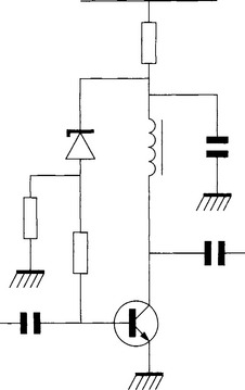
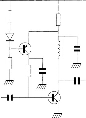
Biasing

MOSFETs are generally easier to bias in PAs than bipolar transistors as they are less susceptible to thermal runaway and do not draw current from their bias circuits. The disadvantage is that MOSFETs have a very wide tolerance on their gate threshold voltage. This means that either the circuit must be set up for each device fitted or some form of active bias control circuit be used. The simplest solution is a variable potentiometer, as shown in Figure 10.4. This can be adjusted to whatever bias current is required. The gate threshold voltage changes with temperature so this may be compensated for by adding a thermistor as shown. Figure 10.5 shows an example of an active bias circuit which needs no alignment to compensate for variation in the gate threshold voltage. This is a good solution for a class A stage which needs a constant current bias. Although the circuit is more complex, the extra components may well be paid for by reduced alignment costs. This circuit may also be used in a variable class mode if the set device current is less than that required for class A operation. In this situation the conduction angle becomes dependent on the drive power. For small drive powers the stage runs in class A. As drive is increased, the transistor starts to be turned off during part of the positive half of the output cycle. This distortion gives a dc component to the output waveform which tries to increase the current consumption. The control circuit will hold the current consumption at its set value by reducing the gate bias voltage. This will continue until the gate bias is at 0 V or the transistor starts to saturate on the negative half of the output cycle. A side effect of the changing conduction angle is that the gain is reduced with increasing drive. This will produce distortion of the RF envelope frequency components within the control loop bandwidth. As to whether this distortion is an advantage or disadvantage depends upon the application. Class A biasing for a bipolar transistor in the HF range can use a bias circuit such as that shown in Figure 10.6. This can be temperature compensated as shown. The layout should be designed to minimize the length of the RF path from the emitter to ground. Any inductance in series with the emitter will reduce the gain of the stage and may compromise the stability. An alternative which can be used if a stabilized supply is in use is shown in Figure 10.7. This method has the advantage of having the emitter connected directly to ground, minimizing stray inductance and allowing use at higher frequencies. A variation of the active bias circuit used for MOSFETs can be used as shown in Figure 10.8. This is much less dependent on supply voltage. A simple Class B bias circuit is shown in Figure 10.9. Close thermal coupling between the diode and RF transistor is necessary to ensure thermal stability. When there is no RF drive the bias current in the transistor will be approximately the same as that flowing through the diode. When drive is applied, the base current will increase. This will cause less current to flow in the diode and hence the bias voltage to drop. It is up to the designer to ensure that the diode current does not drop to zero when the drive is at its maximum if he or she does not want the stage to go into class C operation, with the resulting loss of gain and envelope distortion. Closed loop bias control is not possible as the current is inherently drive dependent. The simplest form of class C bias is shown in Figure 10.10. A resistor can be put in series with the choke which will negative bias the base emitter junction using the base current. If you do use this method, care is required to make sure that the reverse breakdown voltage of the base emitter junction is not exceeded even under worst case conditions. The maximum reverse base emitter voltage is given in Equation 6.

Equation 6

P_in is the input power to the device

R_in is the input resistance of the transistor

R_b is the base bias resistor

I_b is the base bias current

Feedback component selection

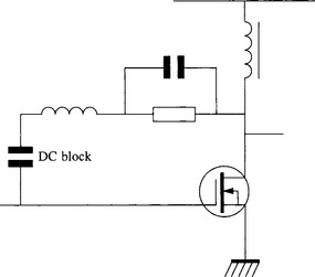
Feedback on a PA stage usually consists of a resistive or complex impedance connected between the drain/collector of the transistor and the gate/base or, less commonly, a resistor between the emitter/source and ground. The latter is to be avoided above HF use and above medium power as the resistance required is usually very low and can easily be swamped by circuit strays, causing a roll off in high frequency gain and power output. Drain to gate feedback is often used to aid stability and control gain in MOSFET stages. Consider the circuit shown in Figure 10.11. The addition of the drain to gate feedback resistor has several effects:

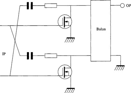
The gain figure from Equation 9 ignores the effect of any reactive components in the circuit, including those within the transistor. The device’s drain to gate capacitance acts in parallel with the external feedback resistance and can be considered as part of a complex feedback network. Adjustments to the circuit can be made to compensate for the effects of the feedback capacitance over a limited frequency range. If the reactance of the feedback capacitance is large compared with the feedback resistor then an inductor in series with the resistor may be all that is required for compensation. A recommended inductor value is given by Equation 11. The resulting network is a two-pole low-pass terminated by the resistor. Depending on the Q of the network, the circuit may produce a gain peak at the value of F_max. When the reactance of the feedback capacitance approaches that of the feedback resistance, then the network in Figure 10.12 can be used. The value of the inductor is two times that given in Equation 11. The capacitor value is the same as that of the feedback capacitance of the transistor. The choice of feedback network is dependent on what degree of gain flatness is required. For push-pull stages there is another way of reducing the effect of feedback capacitance. This is shown in Figure 10.13. This method should be used with care as it effectively introduces positive feedback. The value of the feedback capacitance can vary greatly between samples of a particular device type.

Equation 11

C is the feedback capacitance of the transistor

R_FB is the feedback resistor

F_max is the maximum operating frequency

Unfortunately transistor manufacturers rarely quote minimum feedback capacitance, only typical and/or maximum. For many devices the maximum figure is twice the typical. This suggests, assuming an even distribution, that a good minimum figure is half the quoted typical or a quarter the maximum. In order not to compromise the stability of the circuit, the cross-connected capacitors should not be larger than this minimum figure. The value of the resistors to be used is best found out by experimentation. They are there to maintain high frequency stability.

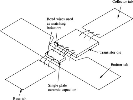
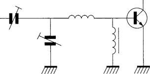
Input matching

When discussing a general class of devices, such as bipolar transistors, the discussion has by necessity to be very vague. There is also a large number of solutions to any particular matching problem. Despite all this, some general comments follow, concerning the type of matching circuits required in PA input matching, and how to design them. In general the input impedance of a bipolar PA transistor is in the order of a few ohms resistive plus a reactive component. At lower frequencies the reactive component is capacitive, and at higher frequencies it is inductive. The cross-over point is in the mid VHF band. The resistive component becomes lower as the power of the stage goes up. At VHF and above, particularly in the higher power devices, impedance matching circuits are included inside the transistor package. These do not usually match direct to 50 O but raise the very low input impedance of the transistor to an impedance which, though still lower than 50 O is much easier to match. The typical construction of such matching is shown in Figure 10.14. The internal matching shunt capacitor has the advantage over external circuits in that one end is directly attached to the same grounding point as the transistor chip. A simple general purpose matching circuit is the two-lumped element variety. The type usually used is the low-pass shown in Figure 10.15. The equations for the reactances are shown in Equations 12 and 13. The inductor and capacitor values derived from them are shown in Equations 14 and 15. These are for matching between two resistances. Any reactive component in the low impedance side can be included in the series reactance of the matching circuit. The Q factor for this circuit is given by Equation 16. Control of the Q factor can be gained by using a three-element matching circuit. The three-element matching circuit shown in Figure 10.16 is commonly used as a test circuit by PA transistor manufacturers. This is because the use of the two variable capacitors enables the circuit to be

Equation 12

R_L is the lower resistance to be matched

R_H is the higher resistance to be matched

Equation 13

Equation 14

Equation 15

Equation 16

adjusted to match a wide range of impedances, but at the expense of a raised Q. If a broadband match is required then other matching circuits should be considered. These include the use of broadband transformers, transmission line elements and more complex lumped element circuits, such as the four-element circuit shown in Figure 10.17. There is very little gain to be had in going beyond a four-component matching circuit. Of course these methods can be mixed as required. A good example of a mixed approach is the combination of a broadband transmission line transformer with lumped element matching. The broadband transformer is limited to impedance transformation ratios which are the squares of integers. When combined with lumped element or further pieces of transmission line matching, this restriction is overcome. The advantage of this approach for large transformation ratios is that the lumped element matching can start from an impedance much closer to that desired and therefore have a much lower Q. Often the lumped element matching components can be included within the broad-band transformer. Practical RF transformers are not ideal and therefore have strays that can be modelled as lumped elements. These strays can be used as part of the lumped element component of the match. As an example of this, consider the 4:1 step-down transformer. This usually has a small series inductance due to non-ideal construction. This inductance can be turned into a lumped element impedance match by the addition of a shunt capacitor. If the capacitor is placed on the high impedance side, the impedance transformation ratio is increased and if on the low impedance side, it is decreased. This transformer if used as a step down from 50 O would ideally be realized using 25 O line, which may not be very practical. A useful trick is to use ordinary 50 O transmission line, thus deliberately increasing the series stray inductance of the transformer, hence increasing the range over which the transformation ratio can be adjusted. The amount of extra inductance created by this trick is obtained using Equation 2. In practice the other contributions such as connecting leads add significantly to this figure so the final arrangement should be built, measured and adjusted before use. There are many other areas where a practical design will probably be forced to depart from ideal RF construction. The trick of good RF design is to use the strays caused by construction limitations to one’s advantage. The limiting factor for lossless broadband matching is the Q of the input impedance of the device. To go beyond this limitation some gain must be sacrificed by the inclusion of resistors external to the device to reduce the Q, or the acceptance of some mismatch. Broadband MOSFET input matching is an extreme example of using resistors to limit the Q of the input match. In this case a shunt resistor is used to provide the majority of the input load. A MOSFET transistor’s input impedance is mainly capacitive and therefore cannot be broadband matched without this shunt resistor. Feedback resistors may also play a significant part in defining the input impedance, and in some circuits form the main part of the input impedance.

Stability considerations

Stability is a very important subject in power amplifier design. It can also be very hard to get right. MOSFETs usually display better stability than bipolar transistors. Due to the non-linear processes present, the stability criteria based on s-parameters (Appendix 2) do not always predict potential oscillations. A bipolar transistor has a reverse biased diode as the collector base junction. This behaves as a varactor diode causing frequency multiplication and division. Frequency division is a common problem in broadband class C stages, and is a symptom of being overdriven or having not enough output voltage available. A MOSFET has a parasitic diode between drain and substrate which can show similar effects. The frequency division aspects are particularly bothersome, as the gain of the devices is usually higher at the lower frequencies. The best way to assess stability is by extensive testing. Stability problems are best overcome by careful layout and the addition of resistive dampers. A base/gate damping resistor should be included from the outset. This is required to limit the Q of any resonance with bias chokes and matching transformers. As an alternative, the damping resistor can be used as a bias injection route, saving on one inductor; however, this is not recommended for bipolar class C stages as the base current drawn will probably cause too much reverse bias of the base emitter junction. As a general rule of thumb, use a resistor value that is four times the base/gate input impedance. If you can get away with damping just at the input, then no output damping should be used as this tends to waste output power. If the oscillations occur at a frequency lower than the required operating range then frequency selective damping on the input and/or output as shown in Figure 10.18 may be used without dissipating too much of the wanted output power in the damping resistor. A technique widely used to stabilize MOSFET stages which have a very large LF gain is to use feedback resistors. Even if they are too high to affect the gain at the operating frequency, they may well successfully prevent oscillations at lower frequencies.

Layout considerations

As a general rule, the higher the frequency and the higher the power, the less you can get away with. Layout should have regard to the impedance at each part of the circuit in question. For low impedance parts of the circuit, minimizing stray series inductance should be of prime concern. For high impedance parts of the circuit, minimizing stray shunt capacitance should be the prime concern. Earth returns, particularly those carrying high RF currents, should be made as short as possible. Sources of stray inductances include component leads, connecting wires to coaxial lines, and lengths of tracking with a characteristic impedance higher than the operating impedance at that point. Sources of stray capacitance include tracking spurs on the PCB and lines of characteristic impedance lower than the operating impedance of the circuit at that point.

Construction tips

The combined requirements of good heat sinking and good RF layout practice often lead to the requirement for a large metal plate associated with the PCB. If it is necessary that the heat sink also provide a good RF earth, the logical extension of this is a thick metal plate bonded to the PCB. The metal plate forms both part of the heat sink and the ground plane. When the heat sink and PCB are separate, repeated assembly and disassembly should be avoided as this can mechanically overstress the bolt-down components. Studmounted transistors should not be soldered to the PCB until they have been bolted down to avoid stressing the leads.

Performance measurements

Power output is usually measured with a power meter. Power meters can be split into two broad groups: those based on thermal heating in a load and those based on diode detectors. Both types will give false readings in the presence of high harmonic levels. The thermal type indicates the total power, including harmonics. The error E due to a second carrier such as a harmonic is shown in Equation 17. If only one harmonic is at a significant level and that level relative to the fundamental is known, then this formula can be used for calculating a correction factor. The diode detector types can indicate high or low depending on the phase of the harmonics relative to the fundamental.

Equation 17

d is the difference between the signal to be measured and the 2nd signal, measured in dBs

Equation 18

Spectrum analysers can be used to measure power without readings being affected by harmonic levels; however, absolute power measurements with spectrum analysers are not as accurate as those by thermal power meters. The harmonic output of a PA stage is simply measured using a spectrum analyser, with a suitable highpower attenuator to bring the carrier power down to a safe level for the spectrum analyser. When the item under test is a PA and harmonic filter combination, the harmonic output may be lower than that produced internally in the spectrum analyser being used to make the measurement. To avoid this problem a test set-up as shown in Figure 10.19 can be used. This uses the notch filter to remove the fundamental of the transmit spectrum, leaving the harmonics to be measured with the spectrum analyser. The attenuator is required to present a reasonable load to the circuit under test. For the higher order harmonics a practical notch filter may be excessively lossy. If this is the case then a high-pass filter can be used in place of the notch for these measurements. Stability into mismatched loads is an important consideration. In the real world, exactly matched loads do not exist - a practical PA will have to tolerate some mismatch. The stability of a PA design will need testing into the worst case VSWR at all phase angles. In nonlinear circuits, supply voltage, temperature, and drive power also will have an effect on stability. Testing the many permutations of these variables is a long and time-consuming job, but for a good PA design it cannot be avoided. A method of presenting a variable phase mismatch and monitoring the output spectrum is shown in Figure 10.20. The phase shifter should be able to present a load that traverses the entire outer ring of the Smith chart at the operating frequency (from short circuit to open circuit and back again). This can be done with a ‘trombone’ (a variable length coax line or ‘line stretcher’) terminated with a short circuit, or a lumped element line stretcher as described in Reference 2

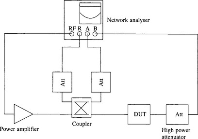
Unlike linear circuits, the input impedance of a PA stage is a function of drive level and supply voltage. Consequently, measurements of input impedance must be made at the design drive level applying in actual use. When the device under test is an unmatched transistor or the existing matching circuit does not give a good match, then the drive from the measurement system may need to be higher than the nominal drive requirement of the circuit in order to get good results. The drive requirements are often beyond the output power capabilities of a network analyser. A typical test set-up for measuring input impedance is shown in Figure 10.21. The device under test should always be tested into its working load, with any output matching circuits in place. With many devices the mismatch between unmatched input and test system is so great that it is not practical to make up for drive loss by just increasing the drive from the test system. In these cases some form of input matching will be needed from the outset. If these matching circuits are characterized on their own beforehand then readings can be translated to get the actual input impedance of the device. Because the input impedance of high-power stages is generally just a few ohms, a good choice for a preliminary matching circuit is the 2:1 step-down broadband RF transformer. This gives a working impedance of 12.5 O from a 50 O measurement system. Suitable transformers are described in Chapter 3. Glitches and steps down on the network analyser trace are a sign of instability, either in the device under test or the measurement system. In these cases damping resistors should be added or the drive source should have a low value attenuator added to its output. An indicated impedance which is outside the Smith chart is a sure sign of a potentially-unstable circuit; damping circuits should be added to bring the impedance within the Smith chart. In service an amplifier may have to coexist in proximity to other amplifiers operating on different frequencies, e.g. another transmitter sharing the same antenna mast. In this situation these incoming signals will mix with the signal being amplified in the output stage to produce a range of products on other frequencies. These are known as back intermodulation products or reverse intermods. The level of these intermodulation products will have to be measured to check that they are not going to be large enough to interfere with other radio communications. When testing this in the laboratory one needs to take precautions against intermodulation products being generated in the test equipment and corrupting the results. A recommended test set-up is shown in Figure 10.22. If the levels produced are too high then either a band-pass filter on the output of the PA should be used or the PA should be made more linear.

1. Smith, J. Modern Communication Circuits, McGraw-Hill, New York

2. March/April, Franke, E.A., Noorani, A.E. Lumped-constant line stretcher for testing power amplifier stability. RF Design 1983:48–57.