CHAPTER 9
APPROXIMATIONS OF 1-PERIODIC SOLUTIONS OF PARTIAL DIFFERENTIAL EQUATIONS
In this chapter we introduce basic finite difference operators that approximate space derivatives and spectral derivatives that are based on Fourier theory. Then the method of lines, a very useful approach that consists of approximating the space derivatives but keeping the time continuous, is explained. Under this approach the partial differential equations become systems of ordinary differential equations, and therefore we can use the results of the first part of the book to analyze the model problems.
9.1 Approximations of space derivatives
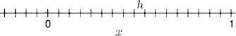
Let M be a positive integer and h = (2M + 1)−1 a grid size. The corresponding grid points are denoted by xj = jh, j = 0, ±1, ±2, …. A grid function fj = f(xj) is simply a function defined on the grid. It is called 1-periodic if
![]()
and therefore any 1-periodic grid function is well defined by its 2M + 1 values f0, f1, …, f2M.
Figure 9.1 Grid.
The most common difference operators approximating d/dx are D+, D−, D0, which are defined by
(9.1) 
and which are called forward, backward, and centered difference operators, respectively. Clearly, if fj is 1-periodic, then D+fj, D−fj, and D0fj are also 1-periodic.
Discretization error and order of accuracy. Let fj denote the restriction of a smooth function f(x) to the grid. The discretization error is the deviation from the exact derivative of the function at a grid point when this derivative is approximated by a difference operator. As the truncation error of a difference approximation to an ordinary differential equation, it can be computed by Taylor expansion. For example, we have
![]()
A similar expansion holds for fj-1. These expansions give
This equations mean that D+ and D− are first-order accurate approximations of the first derivative of f. Because
![]()
we obtain from the error expansions above,
(9.2) ![]()
that is, D0 is a second-order accurate approximation of d/dx.
The difference operator D0 uses the values of the grid function at three consecutive points to compute the derivative at the center point; one says that D0 has a span of three points. One can, of course, write difference operators that use more than three points to construct difference operators with a higher order of accuracy.
Exercise 9.1 Deduce a five-point span centered difference approximation to the first derivative which is accurate of order 4.
Application to Exponentials. Because we intend to use Fourier interpolation, it is important to understand the action of the difference operators on the exponential grid functions e2πiωxj, Because of
![]()
we obtain
(9.4) 
We note that the factor multiplying the grid function e2πiωxj on the right-hand sides is always independent of j. Therefore, the grid function e2πiωxj is an eigenfunction of each of the operators D+, D−, D0. Upon application of any of these operators, the exponential goes over into a multiple of itself.
For fixed xj and j → 0, the left-hand sides of the formula above converge to (d/dx)e2πiωx|x=xj. This follows from the above consideration of the discretization error. Also, if we expand the sine function about zero, we see that the right-hand sides converge to 2πiωxj. Of course, the limits of the two sides are equal since
Remark 9.1 Equation (9.6) says that e2πiωx is an eigenvector of the operator d/dx with eigenvalue 2πiω. If one replaces d/dx by D+ or D− or D0, one obtains the eigenrelations (9.3)–(9.5). A remarkable fact is that only the eigenvalue gets perturbed by this replacement whereas the eigenfunction of each of the discrete operators is precisely the restriction of e2πiωx to the grid. We will see below why this is important for stability analysis.
Approximation for d2/dx2. A very commonly used difference approximation for the second derivative is given by D+D−; this is
![]()
By Taylor expansion,
(9.7) ![]()
which shows that D+D− is a second-order accurate approximation of d2/dx2. Also, from the expression above for D+ and D− applied to e2πiωxj, we obtain
(9.8) 
Exercise 9.2 Find α such that the difference operator
![]()
is a fourth-order accurate approximation of d2 f(xj)/dx2. What is the span of this operator?
9.1.1 Smoothness of the Fourier interpolant
Here we state and prove an important property of the Fourier interpolant introduced in Section 7.3.
Let f(x) be a 1-periodic function and fI(x) be its Fourier interpolant on a given grid xj = hj, j = 0, ±1, ±2, …, where h = 1/(2M + 1) is the mesh size, that is,
(9.9) 
where the Fourier interpolant coefficients ![]() (ω) are computed as in (7.13).
(ω) are computed as in (7.13).
Theorem 9.2
(9.10) ![]()
We emphasize that the constant (π/2)p does not depend on the mesh size h.
Proof: We differentiate fI(x) p times and use the orthogonality of the exponentials (7.2) to get
Applying D+ p times to f(x) at the grid point xj we get, by (9.3),
so that, by (7.16),
9.2 Differentiation of Periodic Functions
If we have a 1-periodic smooth function f(x) we have a Fourier series representation
and we know that the derivative of f(x) can be obtained by multiplying every Fourier coefficient in (9.11) by 2πiω.
Now, assume that we know the restriction of this smooth function to a grid xj [i.e., we know the grid function fj = f(xj)]. How can we efficiently compute a good approximation to the derivative df/dx at the grid points xj?
A good answer is: We first use FFT to calculate the coefficients ![]() (ω) of the Fourier interpolant
(ω) of the Fourier interpolant
We know that fj = fI (xj). Then we differentiate fMF (x) exactly and evaluate on the grid:
The values of dfI(xj)/dx are good approximations of df(xj)/dx and can be computed efficiently by applying IFFT to the coefficients 2πiωf(ω).
9.3 Method of lines
The so called method of lines consists of approximating the space derivatives of a partial differential equation (e.g., by difference approximations) while keeping the time continuous. This semidiscrete approach is very useful to a study of the stability of difference methods of solving the equation. In the method of lines the partial differential equation becomes a system of ordinary differential equations, as we will see. In practice, the method of lines also makes reference to a way of writing computer codes to solve partial differential equations such that the numerical method used to integrate in time can easily be changed without changing the approximation of the space derivatives. In this section we introduce the method of lines by applying it to the model equations of Chapter 8.
9.3.1 One-way wave equation
Consider the initial value problem
We assume that f(x) and therefore also u(x, t) are smooth functions which are 1-periodic in x. We shall only discretize the space dimension but keep the time continuous. Let M be a positive integer, h = (2M + 1)−1 a mesh size thaht defines the grid points xj, j = 0, ±1, ±2, …. We approximate (9.12) on the grid by
We are interested in solutions that are 1-periodic on the grid [i.e., v(xj+2M+1, t) = v(xj, t)], so that (9.13) is a system of 2M + 1 coupled differential equations. The easiest way to calculate the solution is to use essentially the same procedure as that used in Chapter 8.
We start with simple wave solutions and use separation of variables, that is, given a frequency ω, we make the ansatz
By Section 9.1, introducing (9.14) into (9.13) gives us
(9.15) 
Here q(ω) = ai(sin(2πωh)/h) is called the amplification factor. Therefore,
that is,
which is a second-order accurate approximation of u(xj, t) on the grid when the initial data function is ![]() is purely imaginary, then
is purely imaginary, then ![]() and the approximation is stable.
and the approximation is stable.
It is important to notice that every mode (i.e. the solution for a fixed frequency ω), satisfies an ordinary differential equation. By (9.13)–(9.18),
One can compare (9.18) with the exact solution (8.5). For low modes (i.e., |ωh| ![]() 1), q(ω) ≃ 2πiωa, and the solution behaves like the exact solution. For high modes,
1), q(ω) ≃ 2πiωa, and the solution behaves like the exact solution. For high modes, ![]() , and q(ω) ≃ 0, the amplitude is preserved, but the phase error becomes large.
, and q(ω) ≃ 0, the amplitude is preserved, but the phase error becomes large.
As our problem is linear, we can now use the results of Section 7.3 and the principle of superposition to solve (9.12) for general initial data. Consider the semi-discretized problem (9.13) with general 1-periodic initial data. The initial data function can be Fourier interpolated on the grid as in (7.11):
Also, the solution can be Fourier interpolated:
By orthogonality of the exponentials [see (7.12)], ![]() . Inserting (9.21) into (9.13) gives, again by orthogonality of the exponentials, exactly the problem (9.16) for each individual frequency ω. By (9.21) the general solution is a superposition of solutions (9.18),
. Inserting (9.21) into (9.13) gives, again by orthogonality of the exponentials, exactly the problem (9.16) for each individual frequency ω. By (9.21) the general solution is a superposition of solutions (9.18),
which is a second-order accurate approximation of u(xj, t) on the grid. By the discrete Parseval’s relation (7.16), and because q(ω) is purely imaginary,
By (9.23) the energy is preserved during time evolution by the semi-discretized equation (i.e., the approximation is stable).
We now consider the one-way wave equation (9.12) with a lower-order term,
which we approximate on the grid by
![]()
Then the amplification factor becomes
![]()
Thus,
![]()
and v(x, t) behaves like the solutions in Chapter 8.
Artificial dissipation. The addition of a dissipative term to the discrete scheme (9.13) can be used to minimize the bad effect of inaccurately computed high-frequency modes. Instead of (9.13), consider the approximation
which is consistent with (9.24) since the added term is proportional to a second derivative multiplied by h, and thus it vanishes formally when h → 0. The amplification factor becomes
(9.26) ![]()
For small |ωh| we obtain in first approximation
![]()
If ω2h → 0, then q → a2πiω and v(x, t) behaves like the solution of the well-posed problem [see (8.4].
If ω2h ![]() 1 (i.e., we consider high frequencies), Re q → ∞ if b < 0 and ω2h → ∞ and the approximation is unstable. If b > 0, Re q → −∞ for high frequencies and the approximation is stable.
1 (i.e., we consider high frequencies), Re q → ∞ if b < 0 and ω2h → ∞ and the approximation is unstable. If b > 0, Re q → −∞ for high frequencies and the approximation is stable.
In applications, high frequencies (i.e., if ω ≥ 1/h) are not calculated with any accuracy; the artificial dissipation term hbD+D−v, b > 0, helps to control these inaccurate high-frequency terms. Unfortunately, the approximation becomes only first-order accurate because the low frequencies are also affected. To prevent loss of accuracy, the standard artificial dissipation term is the fourth order term,
![]()
Now the approximation is second-order accurate.
Exercise 9.3 Prove that the approximation
![]()
to (9.24) is second-order accurate.
The purpose of the method of lines is to have a way to sort out the methods thaht are definitely unstable. For equations with variable coefficients, one uses the principle of frozen coefficients. For example, if in (9.12) a = a(x, t) is a smooth function, one replaces a(x, t) by a(x0, t0) and treats the constant coefficient problem. If, for any (x0, t0), the method is unstable, the method has to be improved. General theory tells us that if the method is stable at (x, t) = (x0, t0), it must be stable in the neighborhood of that point. If a method is stable at all relevant values of (x, t), it can be applied to the variable coefficient problem.
9.3.2 Heat equation
Consider the 1-periodic initial value problem for the heat equation as in Chapter 8:
On the same grid as for the one-way wave equation, we approximate (9.27) by
(9.28) 
and look for 1-periodic solutions on the grid. With the simple wave ansatz (9.14), we again obtain
where the amplification factor is now
This is as in the previous case a second-order accurate approximation of u(xj, t) on the grid when the initial data function is ![]() .
.
All the approximate modes (9.29) with ω ≠ 0 are decaying exponentially with time, so that the approximation is stable. Notice that ![]() small,
small,
![]()
and the solution is dominated by the exact solution (8.10). When |ωh| ~ 1/2, the approximation is not accurate, but this is not important, as both the exact and approximate modes decay, for any t > 0, very fast exponentially.
Each individual mode (9.29) satisfies an ordinary equation
(9.31) ![]()
In complete analogy with the one-way equation, the solution of (9.27) with general 1-periodic initial data (9.20) is obtained, by superposition of simple wave solutions as in (9.22) but with q(ω) given by (9.30). Using the discrete Parseval’s relation, one can prove that the energy E(t) = ||v(xj, t)||2 decays to ![]() ; thus, the approximation is stable.
; thus, the approximation is stable.
We consider now the heat equation perturbed with lower-order terms [see eq. (8.28)]. We study the second-order accurate semidiscrete approximation
![]()
Fourier transforming, we find that
![]()
where the amplification factor is
![]()
Thus, when |ωh| is small, q(ω) = −4π2ω2d + 2πω(a + ib) + c, and the solution behaves like the exact solution of Chapter 8.
9.3.3 Wave equation
We consider our third model problem of Chapter 8, the 1-periodic wave equation
with f1(x + 1) = f1(x) and f2(x + 1) = f2(x). On the same grid as in the previous model problems, we approximate (9.32) by
Again we look for simple wave solutions of the form
Inserting (9.34) into (9.33) gives us
(9.35) ![]()
Therefore, calling q(ω) = 2a[sin(πωh)/h], we have
(9.36) ![]()
and (9.34) gives
(9.37) 
The simple wave solution is then
This solution is a second-order accurate approximation of the exact simple wave solution (8.17). When ωh is small, q(ω) ~ 2aπω and the (9.38) behaves like the exact solution. When |hω| is large, |hω| ~ 1/2, we have q(ω) ~ 4aω compared to the value 2πaω of the exact solution (i.e., the phase error of high modes is large). One can improve the situation by using a higher-order approximation.
9.4 Time Discretizations and Stability Analysis
One-way wave equation. We shall now also discretize time. By (9.19),
(9.39) ![]()
Thus, we have, for every grid point xj, and every frequency ω, an ordinary differential equation which we write in the form
(9.40) ![]()
Assume that we want to integrate in time using a time step k, that is, we discretize time as tn = kn, n = 0, 1, 2, …. We need the chosen method to be stable to integrate all modes. In other words, we need kq(ω) to belong to the stability region of the method for all ω.
For wave propagation problems, the leapfrog method, which we discussed in Chapter 5, is often a very efficient method. Let vn denote the approximation to y(tn). Then
(9.41) ![]()
As q(ω) is pure imaginary, k > 0 can be chosen small enough so that kq(ω) belongs to the leapfrog’s stability region (see Theorem 5.3). Moreover,
![]()
Therefore |q(ω)| < |a|/h, and the condition
implies stability. For condition (9.42), is known as CFL condition,1 the maximum speed of propagation of the completely discretized scheme (i.e., h/k) needs to be higher or equal to the physical speed |a| of the wave. CFL conditions frequently appear as stability conditions in wave propagation problems.
If q(ω) has a real part, kq(ω) cannot belong to leapfrog’s stability region. One can use the modified leapfrog method of Chapter 5. Assume that
![]()
then the modified leapfrog method is
(9.43) ![]()
In Exercise 5.2 we found that this method is stable if kη(ω) ≤ 0 and kξ(ω) < 1.
Exercise 9.4 The approximation (9.25) for the constant coefficient problem (9.12) can be cured to be second-order accurate by tunning the parameter b if one uses explicit Euler to integrate in time. Consider the approximation (9.25) for problem (9.12) and use explicit Euler to integrate in time. Prove that the truncation error
where u(x, t) is the exact solution of(9.12), is
(9.45) 
Therefore, if we choose b = a2k/2h, the method becomes second-order accurate in both space and time. The approximation (9.44) is known as the Lax-Wendroff method.
Heat equation. If we discretize time and use, for example, the explicit Euler meth: od to integrate the equation, stability requires that −2 ≤ kq(ω) ≤ 0, as −4a/h2 ≤ q(ω)) ≤ 0. Then k is chosen so that
![]()
Even when explicit Euler is only first-order accurate, the choice of k proportional to h2 gives an approximation that is second-order accurate in the parameter h.
Exercise 9.5 Consider initial value problem (9.27) with a = 1 and
![]()
![]()
with k = h2/10, where vjn = v(xj, tn) approximates the solution at the grid point xj = hj and time tn = kn. Write a computer program that computes vjn and show plots of the solution at the same times as those for item (a) using h = 1/10.
![]()
at tn = 0.2 as a function of xj. Do you get the resulti expected?
Wave equation. Differentiating (9.38) twice, we get for every mode
(9.46) ![]()
which has the form of an ordinary differential equation,
(9.47) ![]()
Calling vn the approximation of y(tn), the two-step method
is clearly second-order accurate. We want to study the stability of (9.48). As usual, we assume that vn = κn; then
(9.49) ![]()
If −4 < λk2 < 0, this equation has two different, complex, unitary roots, thus giving a stable approximation.
Exercise 9.6 Prove the last assertion.
In our application
![]()
Without loss of generality we assume that the zero-frequency mode (constant mode) is absent, that is,
Then we have 0 < sin2 (πωh) < ![]() , and the stability condition is satisfied if the CFL condition (9.42) is satisfied.
, and the stability condition is satisfied if the CFL condition (9.42) is satisfied.
We have just shown that the completely discretized centered two-step approximation
(9.51) 
is second-order accurate (in both h and k) and stable if the time step is chosen to satisfy CFL condition (9.42) and (9.50) holds.
1From Courant-Friedrich-Lewy.