APPENDIX B

SOLUTIONS TO EXERCISES

SOLUTIONS FOR CHAPTER 1

1.3 Duhamel’s principle and integration by parts give the answer. One gets ₀ = y₀ in the resonance case and ₀ = y₀ − (−1)ⁿP_n⁽ⁿ⁾(0)/(μ − λ)ⁿ⁺¹ in the nonresonance case.

1.4

1.5 (a)

(b)

(c)

1.7 Assume that y(t) is a smooth solution that blowsup when t → T₀ < ∞. By the mean value theorem, for each t such that 0 < t < T₀, there exists a time , with 0 ≤ ≤ t, such that

Taking the limit t → T₀⁻, the right-hand side diverges and then dy/dt diverges at a time . But cannot be strictly smaller than T₀ because the differential equation forbids dy/dt to diverge when y is finite.

1.9 No. By exercise 1.7 for a smooth solution to blowup in finite time, its derivative needs to diverge too, but this is forbidden by the equation since sin(y) is a bounded, function. More explicitly, the differential equation implies that

Integrating, we have

showing that y(t) cannot diverge in finite time.

SOLUTIONS FOR CHAPTER 2

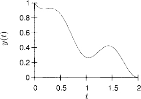
2.1 (a) The analytic solution is

The solution shows an exponentially decaying transient term plus an oscillatory term. The plot of the solution for t [0, 2] is

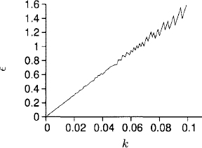
(b) and (c) The plots of the numerical solution and error, for k = 0.1, are

Comparing the graphs, it is clear that the error diminishes by a factor of 10 when the timestep k is diminished by the same factor. This is correct since the global error for the Euler method is of order (k).

2.2 (a) y(t) = 3e^t − 2 − 2t − t².

(b) The plot of (k)is

Clearly, (k) behaves linearly when k is small; therefore, there is a linear bound for (k) but not a quadratic bound.

2.3 By the solution expansion (A.15), we have, for example for ,

2.4 Plots of Q(t), using k = 0.01 on the left and using k = 0.001 on the right:

2.5 By (2.39)–(2.41),

Therefore,

SOLUTIONS FOR CHAPTER 3

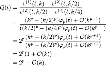
3.2 According to Theorem A.3, the solutions v⁽¹⁾(nk) and v⁽²⁾((2n)(k/2)) satisfy the expansions

(A.1)

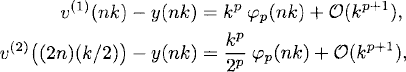
and therefore

(A.2)

Thus, if |v⁽²⁾)((2n)(k/2)) − v⁽¹⁾(nk)| ≤ (2^p − 1)E, we have by (A.2), neglecting terms of order k^p+1,

and therefore

Thus, again neglecting terms of order k^p+1, we have, by (A.1),

in the same time interval in which the condition holds.

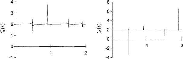
3.3 With k = 0.1 we obtain T = 10.6. The plot of both solutions u⁽¹⁾ (solid line) and u⁽²⁾ (dashed line) are superimposed on the left. The plot on the right is the plot of Q(t).

With k = 0.01 we obtain T = 25.42; the plots are

With k = 0.001 we obtain T = 30.227; the plots are

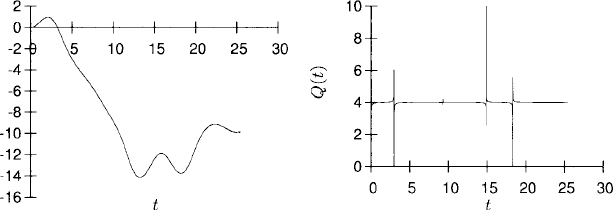
3.4 Plot of the solution:

According to solution expansion (A.15), as the method is fourth-order accurate, the precision quotient Q(t) satisfies

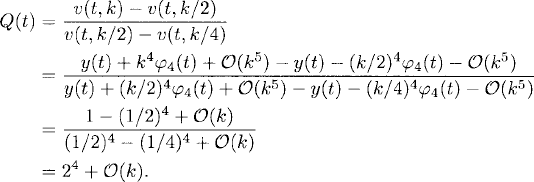
Thus, for k small enough, Q should approach the value 16. The plot of Q(t) obtained is

which shows that the code is working with the accuracy expected.

3.5 When applied to approximate the equation dy/dt = λy, the improved Euler method reads

Then, with μ = kλ = x + iy, the stability region in the complex μ-plane is given by

The plot of this stability region is

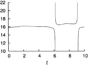
3.6 For the equation dy/dt = iλy, as the time step k > 0, the stability region will be an interval in the imaginary axis. The third-order Taylor method becomes

Calling μ = λk, the stability interval in the imaginary axis is given by the condition

which gives

Therefore, the stability interval is .

3.7 (a) With λ = iμ, μ , we have for the explicit Euler method

and onecan not choose k so that the method is stable.

(b) The modified Euler method proposed will be stable if

On the imaginary axis of the λk-plane, this condition is equivalent, writing λ = iμ, to

or, equivalently,

which holds when (μk)² = 0 (not interesting) or when 0 < (μk)² ≤ (2α − 1)/α². The right-hand side of the last inequality requires that α ≥ 1/2 and reaches its maximum (maximum allowed interval for μk) when α = 1.

3.8 Let y(t) be the exact solution of dy/dt = f(y, t), y(0) = y₀. Thus,

(A.3)

where we have used the equation. Differentiating once more and omitting the dependence on (y, t), we get

(A.4)

(a) Now, by Definitions 3.2 and 3.7 we have, using Taylor expansions of y and f,

In the expression above the terms independent of k cancel out by the differential equation, the linear terms in k cancel out by (A.3), and the cubic terms in k can be simplified by using (A.4), so that the truncation error turns out

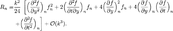
The method is accurate of order 2.

(b) For the method of Heun the analysis is very similar; we get

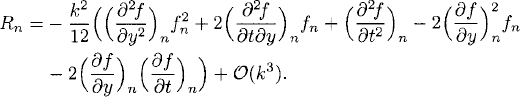
The method is accurate of order 2.

SOLUTIONS FOR CHAPTER 4

4.1 (b)

SOLUTIONS FOR CHAPTER 5

5.2 Proposing v_n = κⁿ, equation (5.17) with F(t) = 0 implies that

whose solutions are, calling x = kη and y = kξ,

The method will be stable if there are two different roots with |κ| ≤ 1. Thus, if x² + y² < 1, x ≤ 0 the square root is nonzero and there are two different solutions; moreover,

5.3 The one-step Adams-Bashforth method for the equation dy/dt = λy is

By Taylor expansion of the exact solution

Thus, the truncation error is

It will be (k) if one chooses β = 1, which gives the explicit Euler method.

The two-step Adams-Bashforth method for the equation dy/dy = λy is

Using the Taylor expansions of the exact solution,

the truncation error becomes

Therefore, we need β₀+β₁ = 1 and β₁ = −1/2. The solution is β₀ = 3/2 and β₁ = −1/2, and the two-step Adams-Bashforth for the general equation dy/dt = f(y, t), is then

5.5 By continuity, it is enough to find the roots of p_μ(κ) and check their moduli for only one point in each region of interest. Calculating numerically, we get:

SOLUTIONS FOR CHAPTER 7

7.4 (a) The Fourier coefficients are (ω) = (−1)^ωi/(2πi).

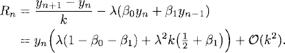
(b) Plots for M = 10; truncated Fourier series on the left and error on the right:

(c) Fourier interpolating polynomial on the left and error on the right:

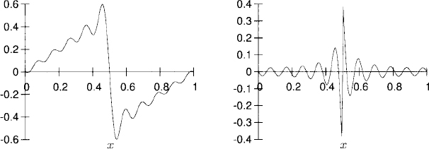
(d) Plots for M = 100; truncated Fourier series on the left and error on the right:

Fourier interpolating polynomial on the left and error on the right:

SOLUTIONS FOR CHAPTER 9

9.1 The approximation has to be antisymmetric around x. Then, writing it as

using Taylor expansion around x and requiring that Df(x) approximates f’(x) to fourth order in h gives equations for A and B whose solutions are and . Thus, the approximation is

9.2 The span is five grid points and α = .

9.3 We have, by Taylor expansion,

Therefore,

and the approximation is second-order accurate.

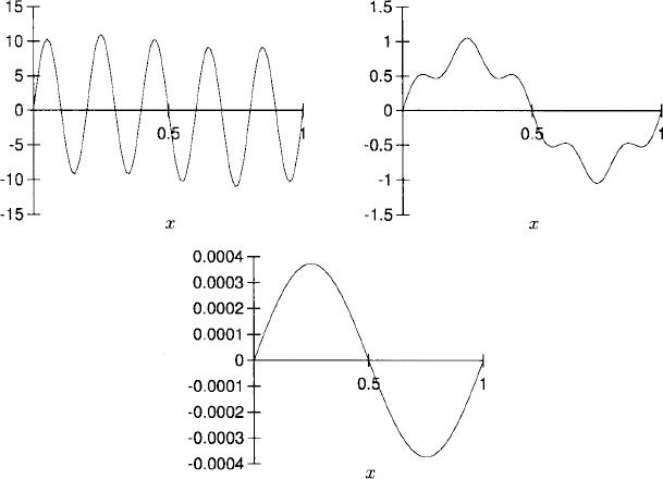
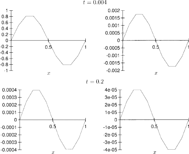
9.5 (a) The exact solution is u(x, t) = sin(2πx)e^−4π2t + 10 sin(10πx)e^−100π2t. The plots of the exact solution at times t = 0, t = 0.004, and t = 0.2 are

(b) and c) The plots of the solution (left plot) and error (right plot) are, for h = 10⁻¹ and k = h²/10,

(d) The plot of Q_j (t = 0.2) is

(e) The plots of the solution (left plot) and error (right plot) are, using h = 10⁻² and k = h²/10,

and the plot of Q_j(t = 0.2) is

9.6 Calling μ = λk², the roots of (9.49) are

If − 4 < μ < 0, the discriminant is μ(1 + μ/4) < 0, and the square root is pure imaginary and different from zero. Thus, we have two different roots with

SOLUTIONS FOR CHAPTER 10

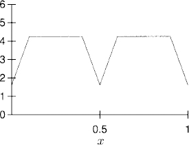
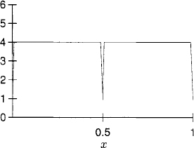
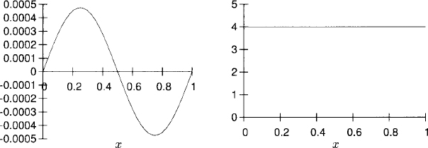
10.2 (a) and (b) Plots for t = 0.002. Solution on the left and Q on the right.

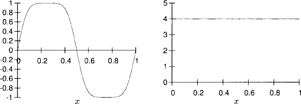
Plots for t = 0.1. Solution on the left and Q on the right.

Plots for t = 0.2. Solution on the left and Q on the right.

10.5 (a) The solution is C¹ smooth and constant along the characteristic lines x+t = const. Thus,

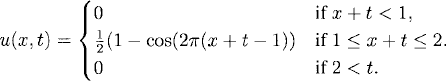
(b) The plots of the numerical solution (left plots) and errors (right plots), at t = 0.5, t = 1.0, and t = 1.5 are, respectively

(c) Q(t = 1) = 3.3513.