CHAPTER 7
Creating Transparency: Formula Structure, Flow and Format
INTRODUCTION
This chapter covers some key ways to enhance the transparency of a model. This represents an important aspect of best practices, since it is one of the major approaches to reducing the complexity of a model. The main themes relate to:
- Putting oneself in the place of an auditor, since doing so helps one to understand the causes of complexity, and hence to determine characteristics of better (less complex) models.
- Drawing clear attention to the location of inputs, calculations and outputs.
- Ensuring that audit paths are clear, and are as short as possible. (Achieving this is also linked to the discussion of workbook structure in Chapter 6.)
- The appropriate use of formatting, comments and other documentation.
APPROACHES TO IDENTIFYING THE DRIVERS OF COMPLEXITY
Taking the Place of a Model Auditor
Perhaps the best way to gain an understanding of what is required to maximise transparency is to do one (ideally both) of the following:
- Review large models that have been built by someone else. When doing so, one is almost invariably struck by their complexity, and the difficulty in understanding their detailed mechanics. It seems that there is unlimited creativity when it comes to building complicated models! Especially by reviewing several models from different contexts, one can start to establish common themes which add complexity unnecessarily. Indeed, many of the themes in this chapter were determined in this way through the author's experience.
- Restructure a clear and transparent model (perhaps built by oneself), with the deliberate aim of making it as hard to follow and as complex as possible, yet leaving the calculated values unchanged (i.e. to create a model which is numerically correct but difficult to follow). It is usually possible (with only a few steps) to turn a small and simple model into one which produces the same result, but with a level of complexity that is overwhelming, and renders the model essentially incomprehensible. This approach is a particularly powerful method to highlight how excessive complexity may develop, and therefore what can be done to avoid it.
The “principle of entropy” applies to models: the natural state of a system is one of disorder, and most actions tend to increase this. Crudely speaking, there are many ways to form a pile of bricks, but the creation of a stable wall, with solid foundations that are sufficient to support the weight above it, requires proper planning and design, the right selection from a range of possible materials, and robust implementation processes. Analogous comments apply to Excel models and their components: the creation of clear and transparent models requires planning, structure, discipline, focus and explicit effort, whereas poor models can be built in a multitude of ways.
Example: Creating Complexity in a Simple Model
Following the discussion in Chapter 3, any action which increases complexity without adding required functionality or flexibility is the antithesis of “best practice”; the use of such complexity-increasing actions is therefore a simple way to highlight both the causes of complexity as well as identifying approaches to reducing it.
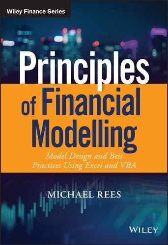
As a simple example, Figure 7.1 shows a small model whose key output is the profit for a business, based on using input assumptions for price, volume and costs. The model should be almost immediately understandable to most readers without further explanation.
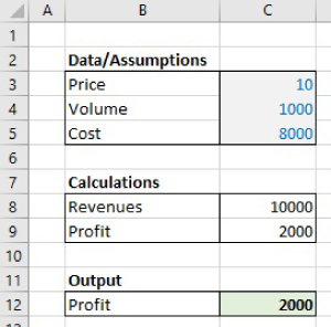
FIGURE 7.1 An Initial Simple and Transparent Model
This model could provide the same results, with a lot less transparency if one were to:
- Remove the formatting from the cells (Figure 7.2).
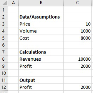
FIGURE 7.2 Initial Model Without Formatting
- Remove the labels around the main calculation areas (Figure 7.3).
FIGURE 7.3 Initial Model Without Formatting and Some Labels
- Move the inputs, calculations and outputs to different areas of the Excel workbook (Figure 7.4). Although it is not shown as an additional explicit Figure, one can imagine an even more complex case, in which items were moved to other worksheets or indeed to other workbooks that are linked. Indeed, although one may consider that the presentation of items in Figure 7.4 looks unrealistic, it is a microcosm of the type of structures that are often inherent in models in which calculations are structured over multiple worksheets.
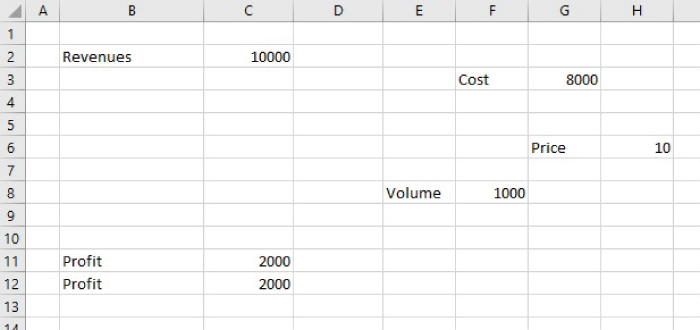
FIGURE 7.4 Restructured Model with Moved Items
Core Elements of Transparent Models
The key points that can be established by reference to the above example concern the techniques that could be applied in reverse, i.e. to start with a model such as in Figure 7.4 (or perhaps the more complex version with some of the items contained in other worksheets or in linked workbooks), and to can transform it into a clear model (i.e. as shown in Figure 7.1). This would require a few core elements, that also encompass many elements of general best practices:
- Using as few worksheets (and workbooks) as possible (see Chapter 6 for a detailed discussion of this).
- Grouping together inputs, as well as calculated items that are related to each other.
- Ensuring that audit paths are generally horizontal and/or vertical, and are as short as possible subject to this.
- Creating a clear direction of logical flow within each worksheet.
- Clearly distinguishing inputs, calculations and outputs, and overall logic and flow (by use of their positioning, format and labels).
These issues (and other related points) are discussed in detail in the rest of this chapter.
OPTIMISING AUDIT PATHS
A core principle to the creation of transparency (and a reduction in complexity) is to minimise the total length of all audit paths. Essentially, if one were to trace the dependency and precedence paths of each input or calculation, and sum these for all inputs, the total length should be minimised. Clearly, a model with this property is likely to be easier to audit and understand than one in which there are much longer dependency paths.
Another core principle is to ensure that audit paths are generally horizontal and vertical, with a top-to-bottom and left-to-right flow.
These principles are discussed in this section. We note that the principles are generally aligned with each other (although may conflict in some specific circumstances), and that there may also be cases where a strict following of the principle may not maximise transparency, with the “meta-principle” of creating transparency usually needing to be dominant, in case of conflicts between the general principles.
Creating Short Audit Paths Using Modular Approaches
An initial discussion of modular approaches was covered to some extent in cover in Chapter 6. In fact, although that discussion was presented within the context of the overall workbook structure, the generic structures presented in Figure 6.1 are more widely applicable (including at the worksheet level); indeed, Figure 6.1 is intended to represent model structures in general.
In this section, we discuss the use of modularised structures within workbook calculation areas. We use a simple example to demonstrate how such structures are often more flexible, transparent and have shorter audit paths than the alternatives.
The file Ch7.1.InputsAndStructures.xlsx contains several worksheets which demonstrate various possible approaches to the structure and layout of the inputs and calculations of a simple model. Despite its simplicity, the example is sufficient to highlight many of the core principles above.
Figure 7.5 shows SheetA1 of the file, which creates a forecast based on applying an assumed growth rate in each period, and with the input assumptions (cells C3:D3) held in a central area, with the calculations based on these being in Row 8 and Row 9.
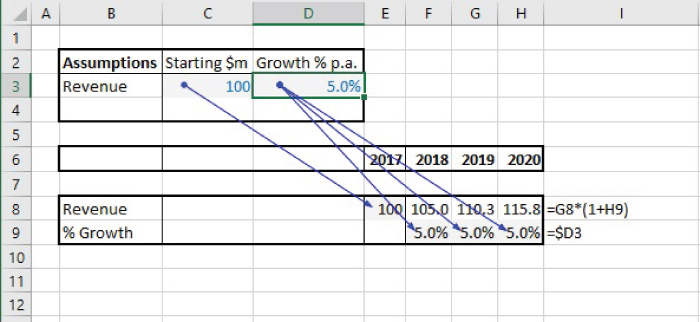
FIGURE 7.5 Simple Forecast with Centralised Assumptions
This is a structure that is frequently observed, and indeed it conforms to best practices in the sense that the inputs are held separately and are clearly marked. However, one can also observe some potential disadvantages:
- The audit paths are diagonal (not purely horizontal or vertical).
- It would not be possible to copy the calculation area, were it desired to add another model component with the same logic (such as a revenue for an additional product, or a cost item). Figure 7.6 shows the incorrect formulae that would result if a copying process were to be conducted (Sheet A2 of the file). (This is because the cell references in the assumptions area and those in the new copied range are not positioned relative to each other appropriately, a problem which cannot be corrected by the use of absolute cell referencing, except in cases where assumptions are of a global nature to be used throughout the model.)
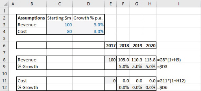
FIGURE 7.6 Centralised Assumptions May Inhibit Copying and Re-using Model Logic
Of course, the formulae in Row 11 and Row 12 can be corrected or rebuilt, resulting in a model shown in Figure 7.7 (and in SheetA3 of the file).
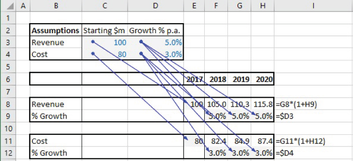
FIGURE 7.7 The Corrected Model and Its Audit Paths for the Centralised Structure
Note that an alternative approach would be to use “localised inputs”. Figure 7.8 (SheetA4 in the file) shows the approach in which the calculations use values of the inputs that have been transferred from the central input area into the corresponding rows of the calculations. Note that the initial calculation area (Row 8 and Row 9) can then be copied (to Row 11 and Row 12), with only the cells in the transfer area (cells C11 and D12) needing to be relinked; the completed model is shown in Figure 7.9 (and contained in SheetA5 of the file).
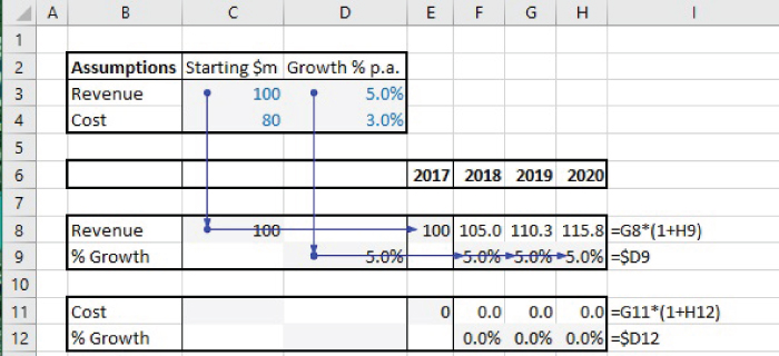
FIGURE 7.8 Centralised Inputs with Transfer Areas to Create Modular Structures
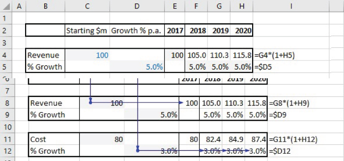
FIGURE 7.9 Audit Paths for Final Model with Centralised Inputs, Transfer Areas and Modular Structures
The approach with transfer areas largely overcomes many of the disadvantages of the original model, in that the audit paths are horizontal and vertical (not diagonal), and the calculation areas can be copied. Note also that the total length of all audit paths in this approach is shorter than in the original model: although a single diagonal line has a shorter length than that of the sum of the two horizontal and vertical lines that arrive at the same point, the original model has more such diagonal lines: for example, in Figure 7.7, there are three diagonal lines from cell C3, whereas in Figure 7.8, these are replaced by a single vertical line and three shorter horizontal lines.
It is also worthwhile noting that, whilst diagonal audit paths can be easy to follow in very small models, they are very hard to follow in larger models, due to the difficulty of scrolling diagonally. Hence the importance of having only horizontal and vertical paths as far as possible.
The above approach, using modularised structures and transfer areas for the centralised assumptions, has the potential advantage that all inputs are shown in a single place. It also has some disadvantages (albeit less significant than in the original model):
- The risk of incorrectly linking the cells in the transfer area to the appropriate inputs.
- The audit paths from the centralised input area to the transfer area may be long (in large models).
- There is a duplication of input values, with those in the transfer area being “quasi inputs” or “calculated inputs”, or “false formulae” (and thus having a slightly ambiguous role, i.e. as to whether they are inputs or calculations).
An alternative approach is therefore to use fully modularised structures from the beginning. Figure 7.10 (SheetB1 in the file) shows the use of a fully modularised structure for the original (revenue only) model.
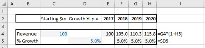
FIGURE 7.10 Fully Modular Structure with Localised Assumptions
Figure 7.11 (Sheet B2 in the file) shows that the original module can easily be copied and the input values altered as appropriate. It also shows the simple flow of the audit paths, and that they are very short.
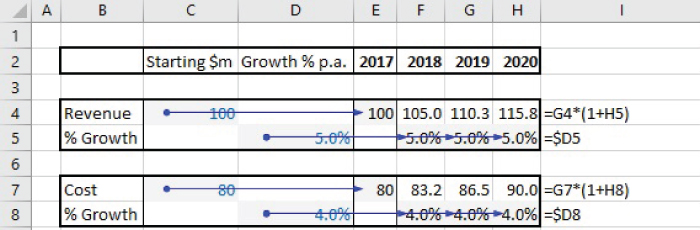
FIGURE 7.11 Reuseable Logic and Short Audit Paths in the Modular Structure
It is also worth noting that the length of the audit paths in this approach is in proportion to the number of modules (since each module is self-contained), whereas in the approach shown in Figure 7.9, the audit paths are not only longer, but also have a total length which would increase according to the square of the number of modules (when in the same worksheet): the audit path from the central area to any new module has a length which includes all previous modules. Therefore in a larger model such as one would typically have in real life, the modular approach affords much better scalability.
In terms of linking this discussion to the structure presented in Chapter 6, we noted that the generic best practices structures (Figure 6.1) may apply at the worksheet level as well as at the workbook level. Thus, the fully modularised structure represents part of a Type III structure (in which only the local data and calculations have been completed, but these have not yet been brought together through the intermediate calculations, such as that of profit as the difference between revenue and cost, nor linked to other global assumptions (such as an exchange rate) that may be relevant in general contexts).
Note that, the placement of “local” inputs within their own modules does mean that not all the model's inputs are grouped together (with only the globally applicable inputs held centrally). However, this should pose no significant issue, providing that the inputs are clearly formatted, and the existence of the modularised structure is clear.
Creating Short Audit Paths Using Formulae Structure and Placement
The creation of short audit paths is not only driven by workbook and worksheet structure, but also by the way that formulae are structured. Generally speaking, the paths used within formulae should be short, with any required longer paths being outside the formulae (and using simple cell references as much as possible), i.e. “short paths within formulae, long paths to link formulae”.
For example, instead of using a formula such as:
one could split the calculations:
In a sense, doing the latter is rather like using a modular approach in which the ranges A1:A15, C1:C15 and E1:E15 are each input areas to the calculations of each module (with each module's calculations simply being the SUM function), and where the final formulae (in cell H18) is used to bring the calculations in the modules together.
Note once again that the latter approach has shorter total audit paths, and also that it is much easy to audit, since the interim summation calculations are shown explicitly and so are easy to check (whereas to detect a source of error in the original approach would be more complex).
Such issues become much more important in models with multiple worksheets. For example, instead of using a formula (say in the Model sheet) such as:
the alternative is to build the summation into each of the worksheets Data1, Data2 and Data3:
and in the Models worksheet, use:
This example highlights the fact that, where dependent formulae may potentially be placed at some distance from their inputs, it is often better to restructure the calculations so that the components required in the formula are calculated as closely as possible to the inputs, with the components then brought together in the final calculation.
Note that, in addition to the general reduction in the total length of audit paths that arise from using this approach, it also less error-prone and sometimes more computationally efficient. For example, when using the original approach (in which the formula sums a range that is on a different sheet), it is more likely that changes may be made to the range (e.g. to Data1!A1:A15), such as adding a new data point at the end of the range (i.e. in Cell A of Data1), or cutting out some rows from the range, or introducing an additional row within the range. Each of these may have unintended consequences, since unless one inspects all dependents of the range before making such changes, errors may be introduced. Where the range has many dependent formula, this can be cumbersome. Further, it may be that a summation of the range is required several times within the model. To calculate it each time (embedded in separate formulae), is not only computationally inefficient, but also leads to the range having many dependents, which can hinder the process of checking whether changes can be made to the range (e.g. adding a new data point) without causing errors.
Finally, note also that when working with multi-worksheet models, it can also be helpful to use structured “transfer” areas in the sheets (to take and pass information to other sheets), with these areas containing (as far as possible) only cell references (not formulae). These are rather like the mirror sheets to link workbooks, as discussed in Chapter 6, but are of course only ranges in the worksheets, rather than being whole worksheets. In particular, cross-worksheet references should generally only be conducted on individual cells (or ranges) and not within formulae.
Optimising Logical Flow and the Direction of the Audit Paths
The way in which logic flows should be clear and intuitive. In principle, this means that generally, the logic should follow a left-to-right and top-to-bottom flow (the “model as you read” principle). This is equivalent to saying that the audit paths (dependence or precedence arrows) would also follow these directions. If there is a mixed logical flow (e.g. most items at the bottom depending on those at the top, but a few items at the top depending on those at the bottom), then the logic is hard to follow, the model is difficult to adapt, and there is also a higher likelihood of creating unintentional circular references.
In fact, there are cases where the strict interpretation of the “model as you read” principle may not be optimal. For example, in forecast models where historic information is used to calibrate assumptions, the flow may often be reversed at some points in the model. Figure 7.12 shows an example of a frequently used structure in which the historic growth rate (Cell D4) is calculated in a “model as you read” manner, whereas the forecast assumptions (in cells E4:G4) are subsequently used in a bottom-to-top flow.
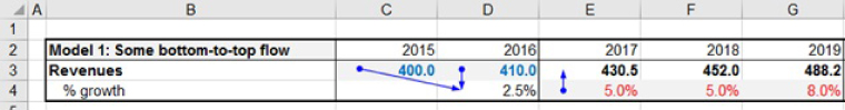
FIGURE 7.12 A Frequent (Often Acceptable) Violation of the “Model as You Read” Principle
Note that the strict adherence to the “top-to-bottom” principle can be achieved. Figure 7.13 shows such a case, which uses historic data (for 2015 and 2016) as well as forecast assumptions. (The formula is analogous to when updating with actuals, as discussed in Chapter 22, using the functions such as ISBLANK.) Thus, whilst the principle has been fully respected, the model is larger and more complex.
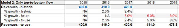
FIGURE 7.13 Strict Adherence to the “Model as You Read” Principle May Not Always Be Best from the Perspective of Simplicity and Transparency
The flow may also need to be compromised where summary calculations are shown at the top of the model, or toward the left-hand side. For example, in a 30-year forecast, in which each column represents a year, one may wish to show summary data (such as total revenues for the first 10 years) toward the left of the model (such as after the revenue label) (see Figure 7.14). Note that the summation calculations (in Column E and Column F) refer to items to their right, and therefore violates the principle. The advantages of doing so include not only the visual convenience of being able to see key summary information toward the left (or the top) of the model, but also that respecting the principle would mean that the summary calculations are placed 30 columns to the right, i.e. in a part of the model that is likely not to be viewed, and which may be overwritten inadvertently (e.g. if adjustments are made to the model's calculations and copied across the columns).
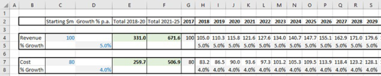
FIGURE 7.14 The Optimal Placement of Summary Information May Compromise the Flow Principle
The flow principle also typically needs to be compromised in financial statement modelling, since the interrelationships between items often mean that trying to achieve a strict top-to-bottom flow would require repetitions of many items, resulting in a larger model. For example, when calculating operating profit, the depreciation charge would need to refer to the fixed asset calculations, whereas the capital expenditure items may be related to the sales level. A pure top-to-bottom flow would therefore not be able to create the financial statements directly; rather, the statements would be created towards the end of the modelling process by referring to individual items that have already been calculated. On the other hand, a smaller model may be possible, in which the statements are determined more directly, but which would require a less clear flow.
IDENTIFYING INPUTS, CALCULATIONS AND OUTPUTS: STRUCTURE AND FORMATTING
It is important to highlight the identity, role and location of the various components of the model. Clearly, some of this can be done through structural methods: for example, in a simple model, one may hold all inputs in a single area, so that their location is clear without much other effort being required. In more complex cases, inputs may be held in several areas (global inputs and those for each module), and so on.
The Role of Formatting
Formatting of cells and ranges has several important roles:
- To highlight the structure, main components and logic flow. Especially the use of borders around input and calculation blocks (and modules) can create more transparency and assist a user's understanding. In that sense, this compensates for the lack of “influence diagrams” in Excel.
- To highlight inputs (see below for a detailed discussion).
- To highlight outputs. Whilst many modellers pay some attention to the formatting of inputs, the benefit of doing so for outputs is often overlooked.
- To draw attention to the occurrence of specific conditions (generally using Conditional Formatting):
- To highlight an error, for example, as detected by an error-checking calculation when the difference between two quantities is not zero.
- If specific criteria are met, such as if the revenue of one product becomes larger than that of another.
- To highlight key values in a data set (such as duplicates, large values etc.); see the options within the Conditional Formatting menu.
- In large tables of calculations in which many elements are typically zero, then it can be useful to de-emphasise cells which contain the value of zero (applications include error-checking calculations, and the triangular calculations for depreciation formulae, discussed in Chapter 18). Conditional Formatting can be used to set the font of zeros to light grey whilst non-zero values remain in the default font. Note that the use of light grey (rather than white, for example) is important to ensure that a user is not led to implicitly believe that the cells are fully blank.
- To assist in model auditing. For example, when using the F5 (GoTo) Special, as soon as one has automatically selected all cells that contain values, one can format these (at the same time) so that there is a record of these.
Colour-coding of Inputs and Outputs
The inputs to a model may in fact have different roles:
- Historical data (reported numbers that will not change, in principle).
- Conversion factors (e.g. years to months, grams to ounces, thousands to millions) or other parameters which would not be meaningful to change. (Arguably, it is acceptable to include such constants within calculations or formulae, rather than placing them in a separate cell that is then referred to by the formulae.)
- Decision variables, whose value can be chosen or selected by a decision-maker. In principle, the values are to be chosen optimally (although they may also be used in a standard sensitivity analysis).
- Uncertain variables, whose values are not directly controllable by the decision-maker (within the context of the model). Beyond standard sensitivity analysis, simulation techniques can be used to assess the range and probability of the possible outcomes.
- Text fields are inputs when they drive some calculations (such as conditional summations which are used in subsequent calculations, or to create a summary report). In such cases, one needs to make sure not only that these fields are spelled correctly, but also that the input is placed in the model only once (for otherwise, sensitivity analysis would give an incorrect result). Thus, an initial text string can be colour-coded or formatted as would be any other input, and placed only once in the model, with all subsequent uses of the text field being made by cell reference links to the unique original entry.
- Databases. In principle, any database entry which is used in a query that feeds a model or a report is an input (as are the field names where Database functions or PivotTables are used). Thus, in theory, most elements of a database should be formatted as inputs (e.g. with shading and colour-coding). In practice, this may not be the optimal way to present a database, due to the overwhelming amount of colour that may result. Further, it is usually implicitly quite clear from the context that the whole database is essentially a model input (and for this reason, this point often escapes explicit consideration entirely). Further, where an Excel Table is used, the overriding of Excel's default formatting for such objects is usually inconvenient, and may be confusing.
- “False formulae”. In some cases, it can be convenient to replace input values with formulae (see Figure 7.9, for example). In such cases, in a sense, the cells containing such formulae nevertheless represent model inputs, not least because the model would be valid if the process were reversed and these formulae were replaced with hard-coded values. (This contrasts with most model contexts, in which the replacement of a calculated field by its value would generally invalidate the model, except for the single base case.)
Regarding outputs, the knowledge of which calculations represent the model's outputs (and are not simply intermediate calculations that are of no interest by themselves) is central to understanding the objectives of the model and modelling process. If the identities of the outputs are not clear, it is in fact very hard for another user to understand or use the model. For example, it would not be clear what sensitivity analysis should be conducted (if at all), or what results should be used for presentation and decision-support purposes. Generically speaking, the outputs include all of the items that are at the very end of the dependency tracing path(s), for otherwise calculations have been performed that are not required. However, outputs may also include some intermediate calculations that are not at the end of dependency paths, but are nevertheless of interest for decision-making purposes. This will be compounded if the layout is poor (especially in multi-sheet models and those with non-left-to-right flows), as the determination of the identity of items at the end of the dependency paths is a time-consuming process, and not one that is guaranteed to find all (or even the correct) the outputs. Therefore, in practice, the identity of the full set of outputs (and only the outputs) will not be clear unless specific steps are taken to highlight them.
The most basic approaches to formatting include using colour-coding and the shading of cells, using capitalised, bold, underlined or italic text, and placing borders around ranges. In principle, the inputs could be formatted according to their nature. However, this could result in a large number of colours being used, which can be visually off-putting. In practice, it is important not to use an excessive range of colours, and not to create too many conditions, each of which would have a different format: doing so would add complexity, and therefore not be best practice. Typically, optimal formatting involves using around 3–5 colour/shading combinations as well as 2–3 border combinations (thin and thick borders, double borders and dashed borders in some cases). The author often uses the following:
- Historic data (and fixed parameters): Blue font with light grey shading.
- Forecast assumptions: There are several choices possible here, including:
- Red font with light grey shading. This is the author's preferred approach, but is not used in cases where there is a desire to use red font for the custom formatting of negative (calculated) numbers.
- Blue font with light yellow shading. This is an alternative that the author uses if red font is desired to be retained to be used for the custom formatting of negative numbers (and calculations).
- Blue font with light grey shading. This is the same as for historic data, and may be appropriate in pure forecasting models in which there is no historic data (only estimates of future parameters), or if the distinction between the past and future is made in some structural (or other) way within the model (such as by using borders).
- Formulae (calculations): Calculations can typically be identified simply by following Excel's default formatting (generally black font, without cell shading), and placing borders around key calculation areas or modules. (In traditional formulae-dominated models, the use of the default formatting for the calculations will minimise the effort required to format the model.)
- “False formulae”: Black font with light grey shading (the colour-code would be changed as applicable if the formula were changed into a value).
- Outputs: Key outputs can use black font with light green shading.
Some caveats about formatting are worth noting:
- The use of capitalised or bold text or numbers can be helpful to highlight key results or the names of main areas. Underlining and italics also have their roles, although their use should be much more restricted, as they can result in items that are difficult to read when in a large Excel worksheet, or when projected or printed.
- Excessive decimal places are often visually overwhelming. On the other hand, if too few decimal points are used, it may appear that a calculated quantity does not vary as some inputs are changed (e.g. where a cell containing the value 4.6% has been formatted so that it displays 5%, the cell would still show 5% if the underlying value changes to 5.2%). Thus, it is important to choose a number of decimal places based on the require figures that are significant.
- A disadvantage of Conditional and Custom Formatting is that their use is not directly visible, so that the ready understanding of the model by others (i.e. its transparency) could be partially compromised. However, cells which contain Conditional Formatting can be found using Home/Conditional Formatting/Manage Rules (where one then selects to look for all rules in This Worksheet) or selected under Home/Find and Select/Conditional Formatting or using the Go To Special (F5 Special) menu.
Basic Formatting Operations
An improvement in formatting is often relatively quick to achieve, and can dramatically improve the transparency of some models. A familiarity with some key short-cuts can be useful in this respect, including (see also Chapter 27):
- Ctrl+1 to display the main Format Cells menu.
- The Format Painter to copy the format of one cell or range to another. To apply it to multiple ranges in sequence (such as if the ranges are not contiguous in the worksheet), a double-click of the icon will keep it active (until it is deactivated by a single click).
- Using Ctrl+* (or Ctrl+Shift+Space) to select the Current Region of a cell, as a first step to placing a border around the range or to format all the cells in the same way.
- To work with borders around a range:
- Ctrl+& to place borders.
- Ctrl+ _ to remove borders.
- To format the text in cells or selected ranges:
- Crtl+2 (or Ctrl+B) to apply or remove bold formatting.
- Ctrl+3 (or Ctrl+I) to apply or remove italic formatting.
- Ctrl+4 (or Ctrl+U) to apply or remove underlining.
- Alt+Enter to insert a line break in a cell when typing labels.
- Ctrl+Enter to copy a formula into a range without disturbing existing formats.
Conditional Formatting
Where one wishes to format a cell (or range) based on its value or content, one can use the Home/Conditional Formatting menu, for example:
- To highlight Excel errors (such as #DIV0!, #N/A!, #VALUE! etc.). This can be achieved using “Manage Rules/New Rule”, then under “Format only cells that contain”, setting the rule description to “Format only cells with” and selecting “errors” (and then setting the desired format using the “Format” button). Dates and blank cells can also be formatted in this way.
- To highlight cells which contain a non-zero value, such as might occur if a cross-check calculation that should evaluate to zero detects an error (non-zero) value. Such cells can be highlighted as above, by selecting “Cell Value is not equal to zero” (instead of “errors”). To avoid displaying very small non-zero values (e.g. that may arise from rounding errors in Excel), one can instead use the “not between” option, in which one sets the lower and upper limits to small negative and positive values respectively.
- Based on dates (using the “Dates Occurring” option on the “Format only cells with” drop-down).
- To highlight low or high values (e.g. Top 5).
- To highlight comparisons or trends using DataBars or Icon Sets.
- To detect duplicate values in a range (or detect unique values).
- To detect a specific text field or word.
- To highlight cells according to the evaluation of a formula. For example, cells which contain an error can be highlighted by using the rule type “Use a formula” to determine which cells to format and then setting the formula to be =ISERROR(cell reference). Similarly, alternate rows of a worksheet can be highlighted by setting the formula =MOD(ROW(A1),2)=1 in the data entry box.
Figure 7.15 shows an example of using Conditional Formatting to highlight dates that occurred in the last seven days. Figure 7.16 shows the use of highlighting values that are less than 1%, and Figure 7.17 shows the highlighting of the top two values only.
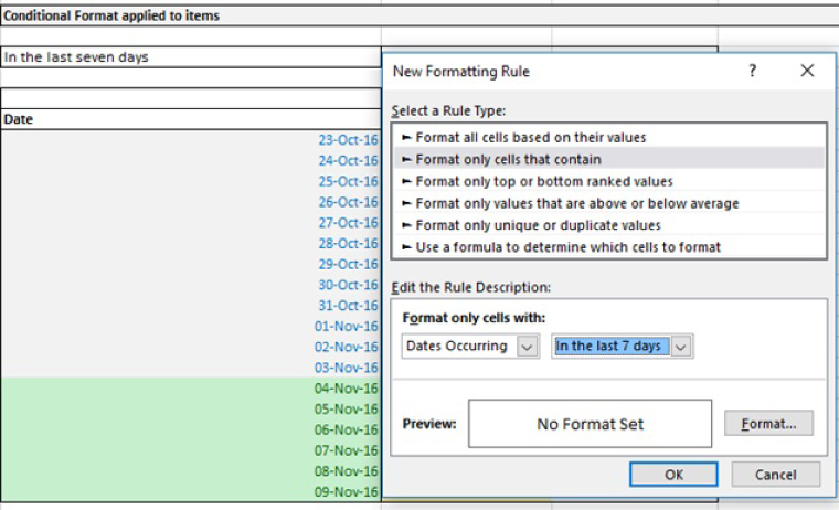
FIGURE 7.15 Example of Conditional Formatting Applied to Dates
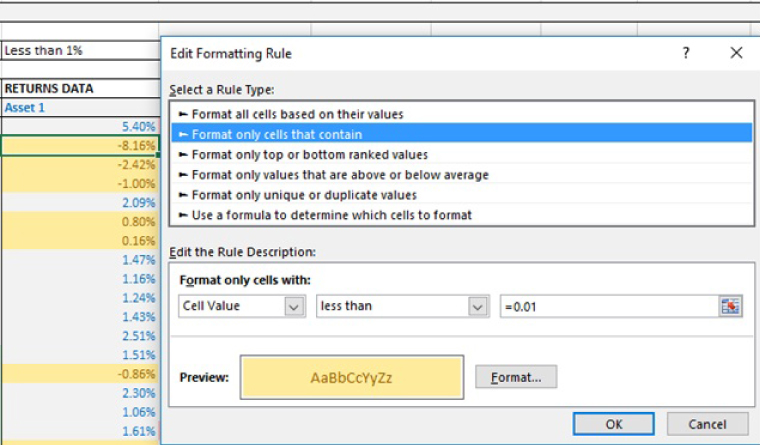
FIGURE 7.16 Using Conditional Formatting to Highlight Values Less Than 1%
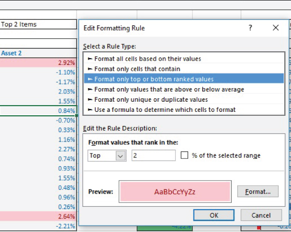
FIGURE 7.17 Using Conditional Formatting to Highlight the Top Two Values
Custom Formatting
Custom Formatting can be used to create customised (bespoke) formatting rules, for example:
- To display negative numbers with brackets.
- To use Continental Formatting, in which a space is used every three digits (in place of a comma).
- To display values in thousands (by using the letter k after the reduced-form value, rather than using actual division), and similarly for millions.
- To Format dates in a desired way (such as 01-Jan-17, if such a format is not available within the standard date options).
The menu is accessible under Home/Number (using the Show icon to bring up the Format Cells dialog and choosing the Custom category); or using the Ctrl+1 short-cut. New formats can be created by direct typing in the Type dialog box, or selecting and modifying one of the existing formats.
The file Ch7.2.CustomFormats.xlsx contains several reference examples. Figure 7.18 shows the case in which negative number are displayed in brackets. Note that the format used for positive numbers is one in which there is a blank space at the end (a blank space before the semi-colon in the format definition), so that the display of units for numbers are aligned if a positive number is displayed above a negative one (or vice versa).
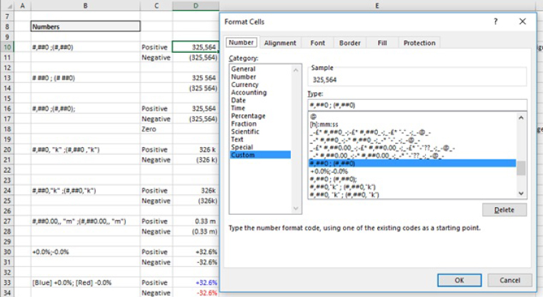
FIGURE 7.18 Examples of Custom Formatting
CREATING DOCUMENTATION, COMMENTS AND HYPERLINKS
It can be helpful to document models, whilst doing so with an emphasis on value-added points, including:
- The key objectives, contextual assumptions and structural limitations (i.e. to the validity of the model or key restrictions on the embedded logic).
- The key input assumptions, and any restrictions on how they may be used (such as requiring integer inputs or where some combinations would not represent valid scenarios).
- Any aspects that could initially appear complex or unintuitive.
Comments or other text may be created in a variety of ways, including:
- Writing general notes as regular text.
- Making a remark in a comment box of a specific cell (Review/Edit Comment menu or right-clicking on the cell to insert a comment).
- In-formula comments, such as =105*ISTEXT(“data from 2017”), or similar approaches using ISNUMBER or other functions (see Chapter 22).
One of the main challenges in using comments is to ensure that they are kept up to date. It is easy to overlook the need to update them when there is a change to the formulae or the input data, or to the implicit contextual assumptions of a model. Some techniques that can help include:
- Using the Review/Show All Comments menu (or the equivalent toolbar short-cut) to show (or hide) all comment boxes, and the Reviewing Toolbar to move between them. This should be done regularly, and as a minimum as a last step before a model is finalised.
- Printing the contents of the comment boxes using Page Layout/Page Setup/Sheet and under Comments selecting whether to print comments at end of the worksheet or as they appear.
- For in-formula comments, one may have to set the model to the Formula View and inspect the comments individually. Alternatively, one may specifically search for ISTEXT, ISNUMBER or other functions and review these individually.
The use of hyperlinks can aid model navigation (and improve transparency), and be an alternative to named ranges. However, hyperlinks often become broken (not updated) as a model is changed. This is disconcerting to a user, who sees part of a model that is not working, and hence will have reduced confidence in its overall integrity. If hyperlinks are used, one should ensure (before sharing the model with others, as a minimum) that they are up to date (Chapter 25 demonstrates some simple examples).