CHAPTER 13
Using GoalSeek and Solver
INTRODUCTION
This chapter provides a description of Excel's GoalSeek, as well as an introduction to Solver. These can both be considered as forms of optimisation tools, in the sense that they search for the input value(s) required so that a model's output has some property or value. Solver's functionality is richer than that of GoalSeek, so that this chapter focuses only on its general application, whilst some further aspects are covered in Chapter 15.
OVERVIEW OF GOALSEEK AND SOLVER
Links to Sensitivity Analysis
Whereas the sensitivity techniques discussed in Chapter 12 can be thought of as “forward-calculating” in nature, GoalSeek and Solver are “backward” approaches:
- GoalSeek (under Data/What-If Analysis) uses an iterative search to determine the value of a single input that would be required to make an output equal to a value that the user specifies.
- Solver determines the values that are required of several inputs so that the output equals some value, or is minimised or maximised. One may also impose restrictions on the allowable value of inputs or calculated values for the set of values to be considered valid. Solver is a free Excel add-in that initially needs to be installed under Excel Options/Add-Ins, and which will then be found under Excel's Data/Analysis menu. It can also be installed (and uninstalled) using the Manage tool for add-ins under Office/Excel Options/Add-ins.
Tips, Tricks and Limitations
Whilst Goal Seek and Solver are quite user-friendly, it is almost always preferable to set up the calculations so that the target value that is to be achieved is zero (rather than some other figure that must be typed into the dialog box). To do this, one simply adds two cells to the model: one containing the desired target value (as a hard-coded figure), and the other that calculates the difference between this value and the model's current output. Thus, the objective becomes to make the value of the difference equal to zero. This setting-to-zero approach has several advantages:
- It is more transparent, since the original value is retained and shown in the model (rather than being a figure that is entered in the GoalSeek dialog box each time that it is run).
- It is more efficient, and less error-prone. If the procedures are likely to be run several times (as is usually the case, not least if other model input values are changed), then it is much easier to enter zero as the desired target value within the GoalSeek or Solver dialogs, rather than to repeatedly enter a more complex value (such as 12.75%).
- It allows for the easier adaptation and generalisation of macros which are recorded when the procedures are run.
- It allows one to use simple techniques to improve accuracy: within the cell containing the difference calculation, one can magnify the raw difference (by multiplication by a number such as 1000), and use GoalSeek to set this magnified difference to zero. This will usually increase accuracy, since the tolerance of Goal Seek's iterative method cannot otherwise be controlled. A similar approach can also be used for Solver, but is usually not necessary, due to its higher inherent accuracy.
When using Solver, some additional points are often worth bearing in mind:
- There must be only one objective, whereas multiple constraints are allowed. Thus, a real-life objective such as “to maximise profits at minimal cost” would generally have to be reformulated. Typically, all but one of the initial (multiple) objectives must be re-expressed as constraints, such as “maximise profit whilst keeping costs below $10m and delivering the project within 3 years”.
- Solver (and GoalSeek) can only find a solution if one exists. Whilst this may seem obvious, a solution may not exist for several reasons: first, one may have too many constraints (or modified objectives). Second, the nature of the model's logic may not capture a true U-shaped curve as an input varies (this is often, but not always, a requirement in optimisation situations). Third, if the constraints are not appropriately formulated, then there can also be many (or infinitely many) solutions; in such cases, the algorithms may not converge, or may provide solutions which are apparently unstable. Fourth, infinitely many solutions can arise in other special cases, for example if one is asked to find the optimal portfolio that can include two assets which have identical characteristics, and so that any amount of one can be substituted for the same amount of the other.
- From a model design perspective, it is often most convenient and transparent to place all the inputs that are varied within the optimisation in a single contiguous range.
PRACTICAL APPLICATIONS
There are many possible applications of such tools, such as to determine:
- The sales volume required for a business to achieve breakeven.
- The maximum allowable investment for a project's cash flows to achieve a specified return target.
- The internal-rate-of-return of a project, i.e. the discount rate for which the net present value is zero (which could be compared to the IRR function).
- The required constant annual payment to pay down a mortgage over a certain time period (which could be compared with the PMT function).
- The mix of assets within a portfolio to sell so that the capital gains tax liability is minimised.
- The parameters to use to define a quadratic (or other) curve, so that it best fits a set of data points.
- The implied volatility of a European option, i.e. the volatility required so that the value determined by the Black–Scholes formula is equal to the observed market price.
Examples of most of these are given below.
Example: Breakeven Analysis of a Business
The file Ch13.1.GoalSeek.Breakeven.xlsx contains a simple model which calculates the profit of a business based on the price per unit sold, the number of units sold and the fixed and per unit (variable) cost. We require to determine the number of units that must be sold so that the profit is zero (i.e. the breakeven volume), and use GoalSeek to do so. (Of course, this assumes that all other inputs are unchanged.) Figure 13.1 shows the initial model (showing a profit of 1000 in Cell C11, when the number of units sold is 1200, shown in Cell C4), as well as the completed GoalSeek dialog box. The model has been set up with the difference calculation method discussed earlier, so that the target value to achieve (that is set within the dialog box) is zero.

FIGURE 13.1 Initial Model with Completed GoalSeek Dialog
In Figure 13.2, the results are shown (i.e. after pressing the OK button twice, once to run GoalSeek, and once to accept its results). The value required for Cell C4 is 1000 units, with Cell C11 showing a profit of zero, as desired.

FIGURE 13.2 Results of Using Goal Seek for Breakeven Analysis
Example: Threshold Investment Amounts
The file Ch13.2.InvestmentThreshold.IRR.xlsx contains an example in which GoalSeek is used to determine the maximum allowable investment so that the post-tax cash flow stream will have an internal rate of return of a specified value. Figure 13.3 shows the GoalSeek dialog to run this. Note that the difference calculation (Cell C12) has been scaled by 1000, in order to try to achieve a more accurate result. The reader can themselves experiment with different multiplication factors, which in principle should be as large as possible (whereas the author's practical experience has been that very large values create a less stable GoalSeek result, and are also generally unnecessary in terms of generating sufficient accuracy).

FIGURE 13.3 Running GoalSeek with a Scaled Target Value for Improved Accuracy
Example: Implied Volatility of an Option
The file Ch13.3.GS.ImpliedVol.xlsx contains the calculation of the value of a European option using the Black–Scholes formula (with six inputs, one of which is the volatility). GoalSeek is used to find the value of the volatility that results in the Black–Scholes-based value equalling the observed market price. Figure 13.4 shows the model and results of running GoalSeek.
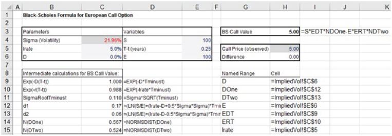
FIGURE 13.4 Using GoalSeek to Determine the Implied Volatility of a European Option
Example: Minimising Capital Gains Tax Liability
The file Ch13.4.Solver.AssetSale.OneStep.xlsx contains an example of the use of Solver. The objective is to find the portion of each of a set of assets that should be sold so that the total proceeds is maximised, whilst ensuring that the realised capital gain (current value less purchase value) does not exceed a threshold at which capital gains tax would start to be paid. Figure 13.5 shows the model, including the data required to calculate the proceeds and capital gains for the whole portfolio (Columns C, D, E), and the corresponding figures if only a proportion of each asset is sold (Columns E, F, G), which are currently set at 100%. Thus the complete selling of all assets in the portfolio would realise £101,000 in proceeds and £31,000 in capital gains. With a capital gain threshold of £10,500, one can see that selling 10,500/31,000 of each asset (approx. 33.9%, as shown in cell H12) would result in the capital gain that is exactly equal to the limit, whilst proceeds would be £34,210 (cell H13). This can be considered as a first estimate (or lower limit) of the possibilities. Thus the objective is to find an alternative set of proportions in which the realised figure is higher than this, whilst respecting the capital gains limit.

FIGURE 13.5 Model for Calculation of Sales Proceeds and Capital Gains
The completed Solver dialog box (invoked, as described at the beginning of the chapter, on the Data tab, after installation) is shown in Figure 13.6. Note that the weights (trial values for the proportions) are constrained to be positive and less than one (i.e. one can only sell what one owns, without making additional purchases or conducting short sales). Figure 13.7 shows the completed model with new trial values once Solver has been run. Note that total proceeds realised are £45,500, and that the constraints are all satisfied, including that the capital gains amount is exactly the threshold value. Of course, the proportion of each asset sold is different to that of the first estimate, whilst the proceeds are higher (£45,500).

FIGURE 13.6 Application of Solver to Optimise Sales Allocation

FIGURE 13.7 Results of Running Solver to Determine Optimum Sales Allocation
It is also worth noting that, since the situation is a continuous one (i.e. the inputs can be varied in a continuous way, and the model's calculations depend in a simple continuous way on these), one should expect that the optimum solution will in principle be one in which the constraints will be met exactly. (If the total portfolio value were below this threshold, this would not apply of course, as it would also not if one constrained the possible values of the inputs in some specific ways.)
Example: Non-linear Curve Fitting
In many situations, one may be required to create (or model) a relationship between two items for which one has data, but where the relationship is not known. One may have deduced from visual inspection that the relationship is not a linear one, and so may wish to try other functional forms. (Where this cannot be done with adequate accuracy or validity, one may instead have to use a scenario approach, in which the original data sets represent different scenarios and the relationship between the items is captured only implicitly as the scenario is varied.)
The file Ch13.5.Solver.CurveFitAsOptimisation.xlsx contains an example of the use of optimisation to fit a curve. A hypothesised relationship (in this case using a logarithmic curve) is created with trial values for each of the required parameters of the relationship. One then reforecasts the calculated values (in this case, the employee productivity) using that relationship. The parameters are determined by setting them as variables that Solver should find in order that the square of the difference between the original and the predicted values is minimised. Figure 13.8 shows the results of doing this. Note that the trial values for the parameters which describe the hypothesised curve (called A, B, C) are in cells C6, C7 and C8 respectively, the predicted values are in Row 11 and the item to minimise (sum of squared differences) in cell K13.
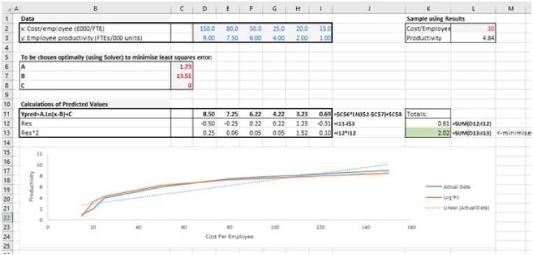
FIGURE 13.8 Results of Using Solver to Fit a Non-linear Curve to Data
It is also worth noting that other forms of relationship can be established in this way, including the determination of the parameters that define the standard least-squares (regression) method to approximate a linear relationship (instead of using the SLOPE and INTERCEPT or LINEST functions, discussed later in the text). One may also experiment with other non-linear relationships, such as one in which the productivity is related to the square root of the cost (rather than its logarithm), and so on. These are left as an exercise for the interested reader.