CHAPTER 25
Lookup and Reference Functions
INTRODUCTION
This chapter discusses Lookup and Reference functions (which, for simplicity, are referred to in the subsequent text only as lookup functions). A good knowledge of these is one of the most important capabilities required to construct intermediate and advanced models.
The chapter starts with examples that relate to basic referencing processes (most of which are either essentially self-explanatory, or have already been covered earlier in the text):
- FORMULATEXT, which shows (as text) the formula in a cell.
- TRANSPOSE, which transposes an array.
- COLUMN (ROW), which returns the column (row) number of a cell or range.
- COLUMNS (ROWS), which finds the number of columns (rows) of a cell or range.
- ADDRESS, which provides a cell reference as text.
- AREAS, which shows the number of areas (separate non-contiguous ranges) in a reference.
The majority of the rest of this chapter is devoted to examples which use the other core functions in additional contexts, including combining matching and referencing processes, and the creation of dynamic ranges and flexible data structures:
- INDEX looks up the value in a specified row and column of a contiguous range (as a one- or two-dimensional matrix). The function also exists in a reference form, where it returns a reference to specified cells rather than to the value of a cell.
- CHOOSE uses one of a set of values according to an indexation number. It is especially useful (compared to other lookup functions) where the arguments are (or may need to be) in a non-contiguous range.
- MATCH finds the relative position of a specified value.
- OFFSET provides the value in a cell that is a specified number of rows and columns from a reference cell or range. It can also be used to return a range of cells (rather than an individual cell) that is a specified number of rows and columns from a reference cell or range.
- INDIRECT returns the range specified by a text string.
- HLOOKUP (VLOOKUP) searches the top row (left column) of a table for a specified value and finds the column in that row (row in that column) that contains that value. It then provides the value that is at a specified row (column) within the table.
- LOOKUP looks up values in a vector or array. In its vector form, it looks for a specified value within a one-dimensional range (of values that must be in ascending order) and returns the value from the corresponding position in another one-dimensional range.
We also briefly mention some of the functions that provide the capability to link to data sets, such as hyperlinks and related topics.
It is important to note that in many of the examples provided, there is generally no unique way to achieve a specific purpose; alternative formulations with different functions may exist. Therefore, we aim to highlight some of the criteria that can be considered when making a choice between various approaches, a topic which was also partly addressed in Chapter 9.
PRACTICAL APPLICATIONS: BASIC REFERENCING PROCESSES
Example: the ROW and COLUMN Functions
The file Ch25.1.ROW.COLUMN.xlsx provides an example of the (essentially self-explanatory) ROW and COLUMN functions (see Figure 25.1). Note that the most frequent practical use would be in the core form, in which the row or column number of a single cell is determined. However, the functions can be used as array formulae to determine the associated values for each cell of a multi-cell range. It is also worthwhile noting (for use later in this chapter) that the functions can be entered in a cell which references itself without creating a circularity (e.g. in Cell B4, the function entered is ROW(B4)).

FIGURE 25.1 Single Cell and Array Formulae use of the ROW and COLUMN Functions
Example: the ROWS and COLUMNS Functions
The file Ch25.2.ROWS.COLUMNS.xlsx provides an example of the ROWS and COLUMNS functions, which are also essentially self-explanatory (see Figure 25.2).

FIGURE 25.2 Example of the ROWS and COLUMNS Function
It is worth noting (for use later in this text) that, whilst ROWS(B3:D7) returns the value 5 (i.e. the number of rows in the range), in VBA the statement Range("B3:D7").Rows refers to the actual rows in the range (not to their number). It is the Count property of this set of rows that would be used to find out the number of rows in a range:
NRows= Range("B3:D7").Rows.CountExample: Use of the ADDRESS Function and the Comparison with CELL
The ADDRESS function returns the address of a cell in a worksheet, given specified row and column numbers. Note that in Chapter 22, we saw that the CELL function could also provide address-related (e.g. address, row, or column number) as well as other information (e.g. its format or type of contents) about a cell.
The file Ch25.3.CELL.ADDRESS.1.xlsx shows an example of the ADDRESS function and the analogous result produced using the address-form of the CELL function (see Figure 25.3).

FIGURE 25.3 Use of ADDRESS and Comparison with CELL
Note (for later reference) that each function can be entered in a cell which references itself without creating a circular calculation. It is also worth noting that the CELL function has the Excel property that it is Volatile. This means that it is evaluated at every recalculation of the worksheet even when its arguments have not changed, which reduces computational efficiency. Thus, the ADDRESS function may be chosen in preference to the CELL function in some cases.
The file Ch25.4.CELL.ADDRESS.4.xlsx contains an example of the use of the ADDRESS function (see Figure 25.4). It uses the last of the function's optional arguments to find the address of a cell in another worksheet of the workbook. In other words, the ADDRESS function is providing (in Cell B3) the full address of Cell B3 of the “Feb” worksheet. A similar result can be obtaining using the address form of the CELL function by explicitly concatenating the text strings. (This approach will be important for some examples of multi-sheet models shown later in the chapter, and discussed in Chapter 6.)
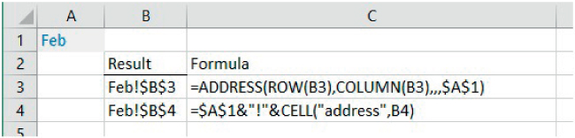
FIGURE 25.4 Finding the Address of Corresponding Cells in Another Worksheet
PRACTICAL APPLICATIONS: FURTHER REFERENCING PROCESSES
Example: Creating Scenarios Using INDEX, OFFSET or CHOOSE
The use of scenario techniques essentially means that the values of several inputs are changed simultaneously. This is usually an extension of sensitivity analysis, which at its core involves changing the value of only one variable. Scenario techniques are useful to begin to capture a wide set of possible outcomes, and to capture dependencies between variables that are believed to exist but which are hard to represent through full mathematical relationships.
Once the scenarios have been defined with explicit data, for any given scenario, the values that are to be used can be looked up from these data sets. The use of lookup processes is an alternative to a “copy and paste” operation (in which model inputs would be manually replaced by the values for the desired scenario), with the function creating a dynamic link between the input scenarios and the model output.
The file Ch25.5.Scenarios.1.xlsx shows an example in which the CHOOSE function is used (Row 6) to pick out the values that apply to the chosen revenue scenario (see Figure 25.5). The desired scenario number is entered in Cell A6, and the references values are linked into the model's subsequent calculations (Row 10 being linked to Row 6). Note that in principle the calculations in Row 6 could instead be placed directly in Row 10. However, for large models such an approach would mean that the CHOOSE function would refer to data that is physically separated from its inputs in a more significant way, and thus be less transparent and more error-prone. Note also that the CHOOSE function requires explicit referencing of the data of each individual scenario.

FIGURE 25.5 Use of the CHOOSE Function to Select the Relevant Scenario Data
Where the scenario data is presented in a contiguous range (such as in the above example), it can be more efficient (in terms of model building and flexibility to add a new scenario) to use the INDEX function to look up the relevant values. (Another alternative is the OFFSET function, although, as a Volatile function, it is less computationally efficient.)
The file Ch25.6.Scenarios.2.xlsx shows the scenario-selection portion of the above example, implemented using each of the CHOOSE, INDEX and OFFSET functions (see Figure 25.6). Note that the CHOOSE function explicitly refers to separate cells, the INDEX function explicitly refers to a contiguous range and the OFFSET function implicitly refers to a contiguous range (by picking out the value that is offset from the date-headers by the number of rows that is equal to the scenario number). Thus, the addition of a new scenario may be easier to achieve if the INDEX or OFFSET functions are used.

FIGURE 25.6 Use of the CHOOSE, INDEX and OFFSET Functions to Select Scenario Data
The file Ch25.7.Scenarios.3.xlsx (see Figure 25.7) shows an extension of the above scenario-selection methods, in which there are scenarios both for cost and for revenue. In principle (e.g. if the dollar signs are implemented appropriately), such scenario-selection formulae may be copied for each desired variable.

FIGURE 25.7 Use of Scenarios for Multiple Model Variables
In practical cases, the scenario data may often be generated in one of two ways:
- By listing first all the revenue scenarios, and then deriving the associated cost scenarios.
- By working scenario-by-scenario (e.g. first the low, then the base, then the high scenario), determining the revenue and cost data with each.
The file Ch25.8.Scenarios.4.xlsx (see Figure 25.8) shows an example in which the structure of the scenario data follows the second of these approaches (whereas Figure 25.7 follows the first). In such a case, the use of the CHOOSE function is often the simplest and most transparent way to achieve the scenario-selection process.

FIGURE 25.8 Use of Scenarios for Non-contiguous Data Sets
Example: Charts that Can Use Multiple or Flexible Data Sources
One may also use the CHOOSE, INDEX, or OFFSET functions to pick out relevant data that is then linked to a graph, and the TEXT (or ADDRESS or other) function(s) may be used to create updating labels for specific graph elements.
The file Ch25.9.Scenarios.5.xlsx shows an example in which the data that feeds the graph, and the graph titles, are updated automatically as the scenario number is changed (see Figure 25.9).

FIGURE 25.9 Scenario Approaches to Creating Graphs
Example: Reversing and Transposing Data Using INDEX or OFFSET
There are many situations in which one may need to reverse or transpose a data set. These include cases where time-series data has been imported from an external source, in “triangle” calculations that arise in depreciation and other similar contexts (see Chapter 18), or when using the results of the LINEST array function in a multiple regression to create predictions (since the coefficients returned by the function are in reverse order to the data sets; see Chapter 21). The INDEX and OFFSET functions can be used to create a dynamic link between an original data set (or calculations) and the reversed or transposed ones.
The file Ch25.10.ReversingTimeSeries.1.xlsx (see Figure 25.10) shows an example. The original data set is shown in Columns B and C, with Column E having been created to provide an indexation reference. The OFFSET function uses this indexation in a subtractive sense; the further down the rows the formula is copied, the less is the result offset from the original data (thus creating the reversal effect).

FIGURE 25.10 Use of OFFSET to Reverse Time-series Data
A similar result can be achieved using INDEX in place of OFFSET; once again, where there is a choice between the two functions, generally INDEX should tend to be favoured, because although OFFSET may have a more appealing or apparently transparent name, the fact that it is a Volatile function reduces computational effectiveness, which can be particularly important with larger data sets and models.
(Note that for simplicity of presentation of the core principles, the examples are shown with only small data sets, but in many practical cases, the number of items would of course be much larger.)
The file Ch25.11.ReversingTimeSeries.2.xlsx (see Figure 25.11) shows an implementation of the INDEX function for the same example.

FIGURE 25.11 Use of INDEX to Reverse Time-series Data
Note that the indexation number created in Column E need not be explicitly placed in the worksheet (it is done so above to maximise transparency of the presentation). Instead, the ROW function could be embedded within the formulae so that the indexation is calculated for each element (the ROWS function could also be used in place of the COUNT function in Cell C2).
The file Ch25.12.ReversingTimeSeries.3.xlsx (see Figure 25.12) shows an implementation of the INDEX function for the same example.

FIGURE 25.12 Using ROW to Create an Embedded Indexation Field
Concerning the transposing of data, as an alternative to the use of the TRANSPOSE array function (Chapter 18), one may use INDEX or OFFSET functions. This similar to the above, except that (to transpose row-form data to column-form), the lookup formulae are written so that as the functions are copied downwards, the lookup process moves across a row.
The file Ch25.13.TranposingWithLookup.xlsx (see Figure 25.13) shows an implementation of this (once again, using an explicit manual approach to indexation in Column B, whereas the ROW and COLUMNS or COUNT functions could be used to create the indexation, either in Column B or embedded within the functions).
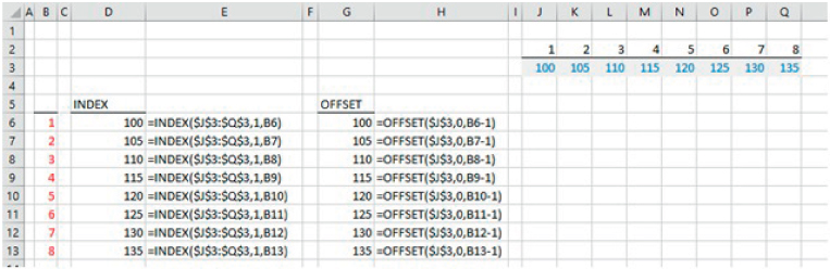
FIGURE 25.13 Using Lookup Functions to Transpose Data
Example: Shifting Cash Flows or Other Items over Time
There are many circumstances in which one may wish to model the effect of a delay on production, on cash flows, or on some other quantity. In such cases, the granularity of the time axis may have an impact on the complexity of the formulae required. In the following, we discuss the following cases:
- Delays whose length is at most one model period (e.g. half a model period).
- Delays whose length is a whole number of model periods.
- Delays whose length could be any positive amount.
The file Ch25.14.TimeShiftVarious.xlsx shows an example of these (see Figure 25.14); the first can be achieved with a simple weighting formula, the second and third by use of INDEX or OFFSET functions. Other simple Excel functions (e.g. IF, AND in the second case and ROUNDDOWN in the third) are also required; the reader can consult the full formulae within the file; for cell I11, the implemented formula is:
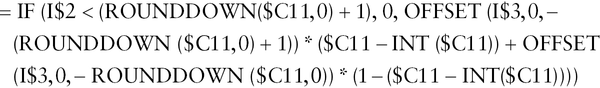

FIGURE 25.14 Various Methods to Shift Cash Flows over Time
Due to their complexity, it is often better to implement them as user-defined functions in VBA (see Chapter 33).
Example: Depreciation Schedules with Triangle Calculations
The file Ch25.15.INDEX.Transpose.Depn.xlsx shows an example in which the INDEX function is used in triangle-type calculations both to transpose and to time-shift the data. The SUMPRODUCT is used to calculate the periodic depreciation (see Figure 25.15). Note that IF and AND statements are used to ensure the validity of the time period, and also that one could not robustly use an IFERROR function in this context (as the INDEX function may sometimes return the first element of a range when the indexation figure is set to zero).
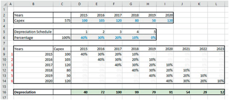
FIGURE 25.15 Using INDEX in a Triangle-type Depreciation Calculation
PRACTICAL APPLICATIONS: COMBINING MATCHING AND REFERENCE PROCESSES
Example: Finding the Period in Which a Condition is Met Using MATCH
It is often important to be able to identify the time period or position in a model at which a condition is met for the first time, for example:
- The first time that revenues of one product are higher than those of another.
- The first time that revenues reach the break-even point, or when those of a declining business drop below such a point.
- The date at which a producing oil field would need to be abandoned as production drops over time as the field becomes exhausted, and future NPV would be negative for the first time.
- The first time at which conditions are met which allow a loan to be refinanced at a lower rate, such as when specific covenant conditions are met.
The MATCH function is powerful in such contexts. Its general syntax is of the form:
Typically, it is most convenient to ensure that the lookup range contains the values of a “flag” variable, i.e. which uses an IF statement to return TRUE (or 1) when the condition is met and FALSE (or 0) otherwise. In addition, it is usually important to use the optional last argument of the function in which a match-type of zero returns the first exact match; if this is omitted, the data in the lookup range needs to be in ascending order and the largest value less than or equal to the lookup value is returned (something which is otherwise often overlooked, resulting in inconsistent values being returned).
The file Ch25.16.RevenueComp.xlsx shows an example applied to finding out when the revenue of one product will overtake that of another, according to the company's revenue growth forecasts (see Figure 25.16). Note that the range F7:O7 contains the calculations of the flag variable, and that the Cell C7 contains the MATCH function. Note also that, if the optional (last) parameter were left empty, then the function would return the position of the last match, not the first (Cell C9). Finally, it is worth reiterating that the function returns the (relative) position (or index number) at which this condition is first met, so that the value in Cell C7 is not the year number (in Row 2) but rather it shows that the match occurs in the eighth position of the data set; the actual year value can be looked up using an INDEX function (Cell C11).
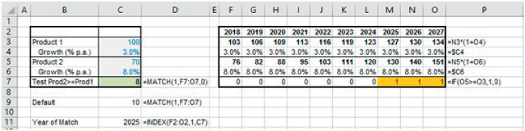
FIGURE 25.16 Using MATCH to Find the Time at Which Revenues Reach a Target
Example: Finding Non-contiguous Scenario Data Using Matching Keys
Earlier in the chapter, we used the CHOOSE function to look up data for scenarios in data sets that were not contiguous, as well as using INDEX or OFFSET when the data is contiguous. Generally, these approaches are the most reliable. Nevertheless, one may encounter models in which more complex (or non-ideal) approaches have been used, and it is worthwhile to be aware of such possibilities.
The file Ch25.17.Scenarios.6.xlsx shows an example in which each scenario is uniquely defined by a text key and this is used to select the appropriate scenario data. The MATCH function finds the position of the scenario within a data set, and the INDEX function is used to look up this data (see Figure 25.17). (As mentioned in Chapter 17, the SWITCH function could also be considered here.)
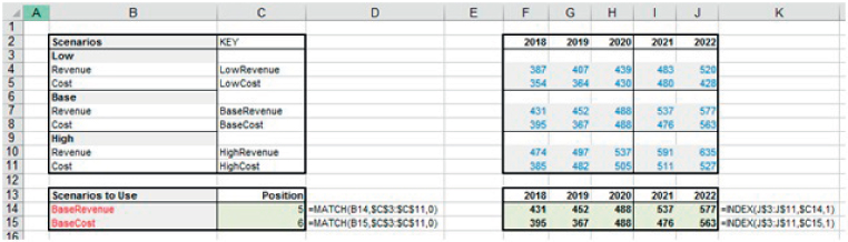
FIGURE 25.17 Using MATCH to Select Data from Non-contiguous Scenarios
Example: Creating and Finding Matching Text Fields or Keys
When manipulating data sets, including combining them or using one within the other, one may need to employ several techniques simultaneously. For example, Text functions may be used to create unique keys (as in Chapter 24) that can be matched together.
The file Ch25.18.Text.CurrencyMatch.1.xlsx shows an example (see Figure 25.18). For the first data set, Text functions are used to manipulate the underlying exchange rate data (in the range B4:C15) to create a unique key for each item (G4:G15), and a similar process is used within the main database. Finally, the position of the matching keys is identified. (The final logical step in the analysis, in which the applicable exchange rates are looked up, is covered in the following example.)

FIGURE 25.18 Using Text Functions and MATCH to Find Data in Currency Database
Example: Combining INDEX with MATCH
As mentioned above, since the MATCH function finds only the relative position of an item (i.e. it returns an indexation number); this generally needs to be used as an input to a further lookup process.
The file Ch25.19.Text.CurrencyMatch.2.xlsx shows the final step in the analysis for the previous example: the INDEX function is used to look up the applicable exchange rates and a calculation performed to find out the total figure in Pounds Sterling (£) (see Figure 25.19).
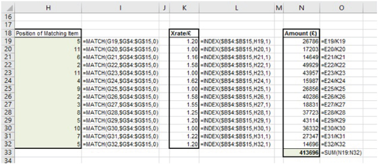
FIGURE 25.19 Combining INDEX and MATCH Processes
Example: Comparing INDEX-MATCH with V- and HLOOKUP
The following examples aim to highlight that the use of INDEX-MATCH combination should almost always be preferred to the use of V- or HLOOKUP functions. This is due to reasons of flexibility, robustness, computational efficiency and superior ease of model auditing.
The file Ch25.20.VLOOKUPINDEXMATCH.1.xlsx shows an example of the use of the VLOOKUP function to provide the appropriate exchange rate data (Figure 25.20). The calculations are correct and seem to offer a sufficient solution to the situation at hand.

FIGURE 25.20 Using VLOOKUP to Find the Relevant Exchange Rate
The file Ch25.21.VLOOKUPINDEXMATCH.2.xlsx highlights that the VLOOKUP function requires values to be matched are placed on the left of the data set. This limits the flexibility in terms of repositioning data sets (copying an initial data set multiple times is an inefficient and error-prone alternative) (see Figure 25.21).

FIGURE 25.21 Limitations to Data Structures When Using VLOOKUP
The file Ch25.22.VLOOKUPINDEXMATCH.3.xlsx highlights that the VLOOKUP function initially uses a hard-coded column number (i.e. Column 2 in this example) (see Figure 25.22). This may lead to the modeller (or another user) making inadvertent errors by adding new columns without adapting the formulae to adjust the column reference. Especially in larger databases and in those which may need to be updated at some point, such errors are frequent and often unobserved; the likelihood of being aware of errors is reduced even further if the data items have similar values (such as columns of salary data in different periods), as errors will not be easily identifiable through the values shown being clearly wrong.

FIGURE 25.22 Error-prone Nature of Hard-coded Column Numbers When Using VLOOKUP
The file Ch25.23.VLOOKUPINDEXMATCH.4.xlsx shows how the above limitation of adding columns in a robust fashion can be overcome by using the MATCH function to determine the column number, so that it is no longer hard-coded (see Figure 25.23). Note that doing so means that a VLOOKUP-MATCH combination has been used to overcome one limitation, another still remains; namely, that the data set needs to be structured with the main lookup column on the left.

FIGURE 25.23 Using MATCH to Create a Flexible Column Number Within VLOOKUP
The file Ch25.24.VLOOKUPINDEXMATCH.5.xslx shows how the INDEX-MATCH combination can be used to create a situation in which the column data can be in any order and new columns may also be inserted without causing errors (see Figure 25.24). Note that the matching and lookup processes can be done separately (Columns G and H) or as a single embedded function (Column K).

FIGURE 25.24 Using INDEX-MATCH in Place of VLOOKUP
In addition to the limitations on the structure of the data set and the error-prone nature of inserting columns, VLOOKUP (and similarly HLOOKUP processes) has other disadvantages:
- Where a key (on the left side of a database) is used to find the values in multiple columns, the implied matching of this key is performed each time, so that computational efficiency is reduced. By performing a single matching step (using MATCH) that is referred to by multiple separate lookup processes, the overall process is more computationally efficient.
- Models containing these functions are often difficult to audit. Partly, this is because the precedents range for any cell containing a VLOOKUP function is the entire (two-dimensional) lookup range, which is often very large. Thus, the backward tracing of potential errors often becomes extremely difficult, and the (digital) file size of the model also very large.
- The data set is hard to restructure, because it is required to be a two-dimensional contiguous range. When developing models, it is usually important to have the flexibility to move data around (for example to minimise audit path lengths by placing data reasonably close to the formulae in which it is used). Moreover, many models have one axis which is logically dominant (such as a time axis in traditional models, or the list of unique identifiers in database models); in such cases a one-dimensional approach to look up processes is often preferable, more flexible and more robust.
The file Ch25.25.VLOOKUPINDEXMATCH.6.xlsx provides an example where each VLOOKUP function is implicitly matching the scenario key (rather than a single match being conducted for each key, followed by the process to look up the values, as shown earlier); as noted above, the looking up of the same scenario multiple times will reduce computational efficiency (recalculation speed) (see Figure 25.25).

FIGURE 25.25 Computation Inefficiency of VLOOKUP When Multiple Items are Looked Up Requiring the Same Underlying Key
Figure 25.26 and 25.27 show simple examples of the dependents- and precedents-tracing processes, showing that every cell in the lookup range is a precedent to every VLOOKUP function that refers to that range.

FIGURE 25.26 Dependency Tracing when VLOOKUP Functions are Used

FIGURE 25.27 Precedents Tracing when VLOOKUP Functions are Used
The file Ch25.26.VLOOKUPINDEXMATCH.7.xlsx shows an implementation of the alternative, which first creates a cell containing the MATCH function to find the relevant row in which data should be taken from (Cell A8), and the INDEX function is driven from individual columns of data. The dependency structure is much clearer and more computationally efficient (see Figure 25.28).

FIGURE 25.28 Greater Transparency and Computational Efficiency of an INDEX/MATCH Approach
Note that although a MATCH function could be embedded within each INDEX function, where the same matching item (i.e. scenario B corresponding to column 2) is used to drive multiple lookup processes (i.e. the functions in Cell C8:G8), it is more computationally efficient to have the MATCH function explicitly in a single cell, so that only a single matching process for each item would happen.
Although the above examples have been shown with reference to the VLOOKUP function, analogous comments apply to HLOOKUP, and so we discuss this with only one specific example.
The file Ch25.27.HLOOKUPINDEXMATCH.8.xlsx shows an example of the error-prone nature of HLOOKUP if new rows are added. Figure 25.29 shows an initial set of formulae which correctly pick out the value of the cost field, and Figure 25.30 shows how the use of a hard-coded row number would lead to an error if a row were inserted without also manually adjusting the row number (i.e. resulting in Row 17 showing revenue data instead of the cost information).

FIGURE 25.29 Use of HLOOKUP to Select Values from a Table

FIGURE 25.30 Potential Errors when a Row is Inserted Within the HLOOKUP Range
Example: Comparing INDEX-MATCH with LOOKUP
The LOOKUP function exists in two forms: the vector form and the array form. Although the Excel Help menu recommends using VLOOKUP or HLOOKUP in place of the array form, the author generally recommends using the INDEX-MATCH approach in place of these! In fact, the vector form is similar to the INDEX-MATCH approach: the function looks for a specified value within a one-dimensional range (of values that must be in ascending order) and returns the value from the corresponding position in another one-dimensional range (if the specified value cannot be found in the first lookup range, matches the largest value that is less than or equal to the specified value; the function returns #N/A where the specified value is smaller than all values in the lookup vector).
The file Ch25.28.LOOKUPINDEXMATCH.xlsx contains an example similar to those above, in which the currency name is first looked up in one field (E3:E5) which provides the position of the relevant currency amount in the other field (C3:C5) (see Figure 25.31).

FIGURE 25.31 Using the Vector Form of the LOOKUP Function as an Alternative to INDEX-MATCH
In summary, the best approach overall would seem to be to use the INDEX-MATCH approach in essentially all cases where VLOOKUP (or HLOOKUP) may otherwise be considered, and even in cases where the vector form of the LOOKUP function could be used. The VLOOKUP (and HLOOKUP) functions create a lack of flexibility, are error-prone, are difficult to audit and are often computationally inefficient. Of course, in simple models (e.g. those containing two columns of data with the lookup values placed in the left column) the use of VLOOKUP would be slightly quicker to implement than the INDEX-MATCH approach. However, it so often arises that initial models are subsequently developed or added to, so that an inappropriate function choice quickly becomes embedded in a larger model and is hard to rectify without significant rework.
The INDEX-MATCH approach is also slightly preferable to the vector form of the LOOKUP function: first, the explicit separation of a single matching step is more efficient where the results are to be used in several subsequent lookup processes (rather than implicitly conducting an embedded match within each). Second, it provides a consistent (and parsimonious) approach to modelling. Third, the LOOKUP function seems to be treated by Microsoft as a legacy function.
Example: Finding the Closest Matching Value Using Array and Other Function Combinations
The lookup functions may be used to find the closest value within a data set that matches an inputted value, by combining the use of several Excel functions. In addition, an approach using array formulae may be considered.
The file Ch25.29.ClosestinList.xlsx shows an example (see Figure 25.32). The requirement is for the user to type a value into Cell C20, with the function sequence determining the value in the list (cells C3:C8) that is closest to this. The calculations on the right-hand side (Columns E rightwards) are the explicit calculation steps, in which the absolute difference between each data point and the input value is calculated (Column F) and the minimum of these is then found (cell I2), the position of this within the data set is found (cell I3) and the value looked up (cell I4). The equivalent calculations can be performed directly as an array formula (without having to create Columns E rightwards), as shown in Cell C21. (Cell C22 shows a variation for reference, in which OFFSET is used to perform the final lookup stage.)

FIGURE 25.32 Finding Closest Matching Values Using Lookup and Array Formula
PRACTICAL APPLICATIONS: MORE ON THE OFFSET FUNCTION AND DYNAMIC RANGES
The OFFSET function can be particularly useful to create formulae that refer to ranges which are flexible, in the sense that either the size or location adjusts based on inputs or calculations. In the following examples, we show three main variations:
- Where the referenced range is a cell and the returned reference is a cell.
- Where the referenced range is a range and the returned reference is a range (without using the optional height and width arguments of the function).
- Where the referenced range is a cell and the returned reference is a range (by using the optional height and width arguments of the function).
Note that the INDEX function also exists in a reference form (rather than the array form used earlier in the chapter), and as such can often be used to perform operations similar to some of those shown here. However, we find that the use of such a form is typically less flexible and less transparent than other formulations, so it is not discussed further in this text.
Example: Flexible Ranges Using OFFSET (I)
A simple example of the use of OFFSET to create dynamic ranges is to sum a range from one point to another. For example, one may wish to sum the values along a row between two cells whose location may vary (e.g. where the starting and ending cells are either model inputs or are determined from calculations.)
The file Ch25.30.DynamicRange.SumColumn.1.xlsx shows an example in which the user defines which part of a series of cash flows are to be included in the summation, by providing the starting and end period as inputs (see Figure 25.33). The formula in Cell C7 is:
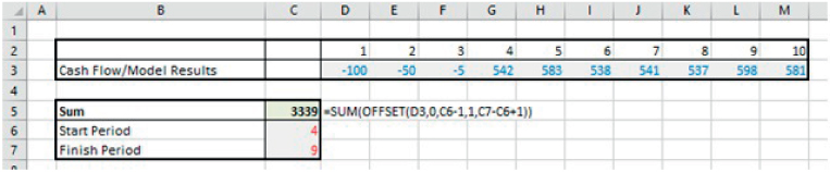
FIGURE 25.33 Using OFFSET to Sum Between User-defined Cells
In this formula, the last two arguments of the OFFSET function (which are optional function arguments) are used to create a range of height one and width six, starting from the fourth cell in the range D3:M3 (i.e. based on the user-defined inputs in cells C6 and C7).
The file Ch25.31.DynamicRange.SumColumn.2.xlsx shows an extension of this in which the starting point for the summation is determined from the calculations in the model, specifically to sum the cash flows in the six-year range starting from the point at which the first positive cash flow is detected (calculated by the array function in Cell C6). Thus, in a real-life model in which the cash flows in Row 3 are determined through calculations based on other inputs, the starting point for the summation would move dynamically as input values were changed (see Figure 25.34). Note that similar calculations could be done to sum the range backwards from a starting point; this might be required in tax calculations where only a certain number of prior years of tax losses can be carried forward.

FIGURE 25.34 Using OFFSET to Sum Between Calculated Cells
Example: Flexible Ranges Using OFFSET (II)
Another simple example of creating flexible range using OFFSET is a formula which sums the items in the rows above it, in such a way that if a row is introduced, the summation would still be correct.
The file Ch25.32.DynamicRange.SumRowsAbove.xlsx shows an example (see Figure 25.35). Note that this example is of a legacy nature in Excel. In older versions, the introduction of a new row between the last item and the sum formula (i.e. between the Row 10 and 11 as shown) would have resulted in a SUM formula (shown initially in Cell C11, but which would then be in Cell C12) that would not include this new row. On the other hand, the formula in F11 automatically sums the items until the row immediately above the formula, and so will adapt automatically. Note that recent versions of Excel will automatically adjust the summation formula (C11) by extending its range when a row is inserted and a value entered.

FIGURE 25.35 Using OFFSET to Sum Rows Above
Example: Flexible Ranges Using OFFSET (III)
Whereas the above examples using OFFSET focused on changing the size of a referenced range, other uses relate to changing the data set that is being referred to. One application is in the calculation of correlation matrices in which there are several variables, or for which the data of an additional variable may be added at some future point. When using reference formulae, such as CORREL(Range1, Range2), where Range1 and Range2 are direct input ranges, the formula created in an initial cell cannot be copied to the rest of the correlation matrix (since it is not possible to create a single formula with the correct $ structure (for absolute cell referencing) that can be copied in both the row and column directions). On the other hand, the OFFSET function can be used to create a single formula in which the ranges adapt automatically, and can therefore be copied to the full range of the matrix. Except for very small matrices (such as 2×2 or 3×3) this saves time and ensures that subsequent additions to the data set can also be rapidly incorporated.
The file Ch25.33.DynamicRange.Correl.xlsx shows an example (see Figure 25.36). Note that the formulae using the OFFSET function themselves create ranges (and not values). Therefore, they must be embedded within another function (and cannot be placed explicitly in an Excel cell). Thus, the formula in Cell F9 is:

FIGURE 25.36 Creation of a Correlation Matrix Using a Single Formula
Example: Flexible Ranges Using OFFSET (IV)
The file Ch25.34.DynamicRange.Languages.xlsx shows a final example of the use of the OFFSET function to translate Excel functions from one language to another.
As a starting point for the discussion, Figure 25.37 shows the possible use of the VLOOKUP function if one is translating from a language that is always on the leftmost column of the data set. As discussed earlier, the INDEX-MATCH approach provides more flexibility irrespective of how the data is laid out. However, these examples are based on the idea that the two languages are both fixed and that the translation is in a known order (i.e. English to German in these examples).

FIGURE 25.37 Translation Between Two Fixed Languages
In Figure 25.38, we show an example from the same file, in which the translation can be done from any language to any other. In this case the MATCH function is used to determine the relative column position of each language within the data set (e.g. German is the second column). A key formula is that in cell I6 (showing the value 60), which is:

FIGURE 25.38 Translation Between Any Two Languages
In this formula, the position of the word to be translated (here: Anzahl2) is looked up within a column range, which is itself determined as that which is offset from the first column of the data set in accordance with the language in which this word exists.
PRACTICAL APPLICATIONS: THE INDIRECT FUNCTION AND FLEXIBLE WORKBOOK OR DATA STRUCTURES
Example: Simple Examples of Using INDIRECT to Refer to Cells and Other Worksheets
Where a text field can be interpreted by Excel as the address of a cell or range of cells, the INDIRECT function can be used to find the values in that cell or range. For example, the statement:
would refer to Cell C2, as if one had used the direct cell reference formula:
The file Ch25.35.INDIRECT.Basic.xlsx shows some examples of these. Figure 25.39 shows a simple example in which the value in Cell C2 is required in later parts of the model (Column E).

FIGURE 25.39 Basic Application of the INDIRECT Function
In Figure 25.40, we show an extended example, in which the cell reference C2 is either hard-coded (Cell E6) or is determined using various forms of the ADDRESS or CELL function.

FIGURE 25.40 Combining INDIRECT with ADDRESS or CELL Functions
In Figure 25.41, we show a further example, in which the data is taken from another worksheet, using both a direct reference to the cell in the other worksheet and an indirect one.

FIGURE 25.41 Direct and Indirect Referencing of Data on Another Worksheet
Finally, Figure 25.42 shows an example of the function being applied where the input text field identifies a range, rather than a single cell.

FIGURE 25.42 Use of a Text Argument as a Range Within the INDIRECT Function
These approaches are used in practice in the next examples.
Example: Incorporating Data from Multiple Worksheet Models and Flexible Scenario Modelling
One of the most powerful applications of the use of the INDIRECT function is to create “data-driven” models, in which there are several worksheets containing underlying data, and in which the user specifies the worksheet that data is to be taken from. The function is used to refer to the values on the specified worksheet. Such an approach allows new data worksheets to be added (or old ones deleted) with minimal effort or adjustment, as long as the data worksheets have a common structure.
An important specific application of this approach is in scenario modelling, where the number of scenarios is not known in advance. If the number is fixed (say, three or five), then separate data worksheets for each scenario could be built in the model, and the data selected using a direct cell reference approach (such as with the CHOOSE or INDEX function). Where the number of scenarios is not known, then this multi-sheet approach allows a scenario sheet to be added (or deleted).
The file Ch25.36.INDIRECT.DataSheetSelection.xlsx contains an example of this. Note that there are four underlying data worksheets in the original model, as well as a data selection worksheet (named Intermediate). The user defines which worksheet the data is to be taken from (by entering its name in Cell A1 of the Intermediate worksheet). The formulae in the Intermediate worksheet each find the reference of their own cell, before the INDIRECT function is used to find the value in a cell with the same reference but in the selected data worksheet (see Figure 25.43). (For illustrative purposes, both CELL and ADDRESS have been used.)

FIGURE 25.43 Using INDIRECT to Incorporate Data from a Specified Sheet
Note that:
- In general, in a real-life model, the Intermediate worksheet will itself be used to make a (direct) link to (or “feed”) a model worksheet. The model worksheet does not then need to have the same structure as the Intermediate worksheet, nor as the data worksheets. The use of this intermediate step (i.e. bringing data indirectly from the data sheets to an Intermediate worksheet and from there to a model sheet) allows one to ensure a strict consistency between the cell structure of the Intermediate worksheet and those of the underlying data worksheets; this is required in order to have a simple and robust indirect referencing process.
- Although it is important generally that the data worksheets have a similar structure to each other, in some more complex practical cases, the data worksheets may also contain calculations which are specific to each one (and different from worksheet to worksheet). However, providing there is a summary area in each sheet which has a structure that is common to the other data worksheets, then the above approach can still be used.
These topics are closely related to the data-driven modelling approaches that were discussed in detail in Chapter 5 and Chapter 6.
Example: Other Uses of INDIRECT – Cascading Drop-down Lists
There are of course many possible uses of the INDIRECT function other than those above.
The file Ch25.37.INDIRECT.DataValidation.SequentialDropDowns.xlsx contains an example of context-sensitive drop-down lists (or cascading menus). The user first selects a main category of food, after which the INDIRECT function is used to create a new drop-down, which lists only the relevant items within the chosen category (see Figure 25.44). Note that this is achieved using the category names as Excel Named Ranges which each refer to the list of items within that category (e.g. ProteinSource is the range C5:F5), and using the INDIRECT function within a Data Validation list (for Cell C9), so that the list refers only to items in that category.

FIGURE 25.44 Sequential Drop-downs Using INDIRECT
PRACTICAL EXAMPLES: USE OF HYPERLINKS TO NAVIGATE A MODEL, AND OTHER LINKS TO DATA SETS
In this section, we briefly mention some functions that can be used to provide links to data sets:
- HYPERLINK creates a short-cut or jump that can be used to insert a hyperlink in a document as a function. The link may be either a named range within the Excel file, or more generally a link to a document stored on a network server, an intranet or the Internet. The function has an optional parameter so that the displayed link may also be given a “friendly name”. This is similar in overall concept to the use of the Insert/Hyperlink operation, except that this latter operation results in a direct link (rather than a function which returns a link).
- GETPIVOTDATA returns data stored in a PivotTable report.
- RTD retrieves real-time data from a program that supports COM automation.
Example: Model Navigation Using Named Ranges and Hyperlinks
The file Ch25.38.Hyperlinks.NamedRanges.xlsx shows an example of the use of both the HYPERLINK function and of a hyperlink inserted using the Insert/Hyperlink operation, in each case to reference a part of the model (Cell A1) defined with a named range (DataAreaStart) (see Figure 25.45).

FIGURE 25.45 Comparison and Use of HYPERLINK Function or Insert/Hyperlink Menu