CHAPTER 27
Selected Short-cuts and Other Features
INTRODUCTION
This chapter presents a list of the key short-cuts that the author has found to be the most useful. Most of these are self-evident once they have been practised several times, so that only a few screen-clips are shown to demonstrate specific examples. The mastering of short-cuts can improve efficiency and speed of working. Therefore, each modeller should develop a good familiarity with those short-cuts that will be most relevant to them, and have a general understanding of the wider set available should they be useful in specific circumstances. It is worth noting that some of the short-cuts become particularly relevant when recording VBA code, as they allow to capture the code for operations that would not otherwise be evident. There are of course short-cuts available in Excel that are not covered in this chapter, and the reader may conduct his or her own research in this regard, perhaps using the list in this chapter as an initial check-list. The chapter also briefly mentions some of the Excel KeyTips, as well as some other potentially useful tools, such as Sparklines and the Camera.
KEY SHORT-CUTS AND THEIR USES
The key short-cuts we cover are structured into their main categories of application:
- Entering and modifying data and formulae.
- Formatting.
- Auditing, navigation and other items.
Note that, on a UK keyboard, some of these short-cuts (such as Ctrl+&) would require one to use the Shift key to access the relevant symbol (such as &); in such cases the Shift is not considered as part of the short-cut.
Entering and Modifying Data and Formulae
Core short-cuts for copying values and formulae, and correcting entries, include:
- Ctrl+C to copy a cell or range, Ctrl+X to cut, Ctrl+V to paste.
- Ctrl+Z to undo.
- When editing a formula in the Formula Bar, F4 implements absolute cell references (e.g. place a $ before a row reference); repeated pressing enables one to cycle through all possible combinations ($ before row and columns, and removal of $). The ease of applying the short-cut may lead to the creation of “over-dollared” formulae, i.e. ones in which the $ symbol is inserted before both the row and column references, whether only one or the other is required; this will typically result in formulae that cannot be correctly copied to elsewhere in the model.
- A formula (as well as its cell formatting) can be copied from a single cell into a range by using Ctrl+C (to initiate the copy procedure) and then, with this cell selected, either:
- Pressing Shift and simultaneously selecting the last cell of the range in which the formula is desired to be copied, followed by Ctrl+V.
- Pressing F8 and (following its release) selecting the last cell of the range in which the formula is desired to be copied, followed by Ctrl+V.
- Using Ctrl+Shift+Arrow to select the range from the current cell to end of range in the direction of the arrow, followed by Ctrl+V.
- A formula (but not its formatting) can be copied from a single cell into a range by creating the formula in the first cell of the range, then using any of the techniques mentioned above to select the range in which the formula is to be copied, and then – working in the Formula Bar – entering Ctrl+Enter (or Ctrl+Shift+Enter for an array formula). This is particularly useful when modifying models which are already partially built and formatted, as it does not replace the formats that have been set in the cells to be overwritten. Figure 27.1 shows an example, just prior to using Ctrl+Enter, i.e. the formula has been created in the Formula Bar and the range has been selected.

FIGURE 27.1 Copying a Formula Without Altering Preset Formatting
- A formula can be copied down all the “relevant” rows in a column by double-clicking on bottom right of cell; the number of rows that are copied into will be determined by the rows in the Current Region of that cell (i.e. in the simplest case, to the point where the adjacent column also has content).
- Ctrl+' (apostrophe) can be used to recreate the contents of the cell directly above (rather than copying formula which would then generally alter the cell references within it). One case where this is useful is where one wishes to split a compound formula into its components, showing each component on a separate line. One can initially repeat the formula in the rows below, and delete the unnecessary components to isolate the individual elements. This will often be quicker and more robust than re-typing the individual components. As a trivial illustrative example, the individual components within a formula such as:
could be isolated in separate cells before being summed.
When creating formula, the following are worth noting:
- After first typing a valid function name (e.g. such as “MATCH”):
- Ctrl+Shift+A shows the argument names and parentheses required for a function, and places these within the Formula Bar; an example is shown in Figure 27.2.
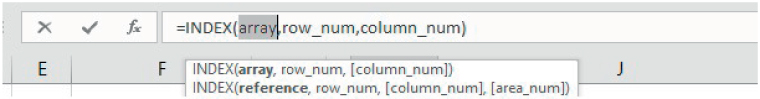
FIGURE 27.2 Invoking Function Parameters Within the Formula Bar Using Ctrl+Shift+A
- Ctrl+A invokes the Insert Function dialog, allowing for the function's parameters to be connected to cells more easily.
- Ctrl+Shift+A shows the argument names and parentheses required for a function, and places these within the Formula Bar; an example is shown in Figure 27.2.
- Defining and using named ranges:
- When creating formulae that require referencing ranges that have been named, pressing F3 when in the Formula Bar will provide a menu of the names that can be used (i.e. of workbook and worksheet-scoped names). Figure 27.3 shows an example of a formula being built by pressing F3 to show the list of named areas (and selecting them as relevant).

FIGURE 27.3 Building a Formula by Invoking the List of Named Ranges
- Ctrl+F3 can be used to invoke the Name Manager to define a named range.
- Ctrl+Shift+F3 can be used to create range names from labels (although the author generally recommends to not do so; taking time to reflect on the most appropriate structure and hierarchy of named ranges, as well as their scope, is usually very important, and an automatic naming will often not generate such a set of names).
- Ctrl+K will insert a hyperlink, include a link to named range, and can be a useful model navigation and documentation tool.
- When creating formulae that require referencing ranges that have been named, pressing F3 when in the Formula Bar will provide a menu of the names that can be used (i.e. of workbook and worksheet-scoped names). Figure 27.3 shows an example of a formula being built by pressing F3 to show the list of named areas (and selecting them as relevant).
- Shift+F3 invokes the Insert Function (Paste Function) dialog (arguably, doing so is not any quicker than simply clicking on the button directly).
Formatting
The use of appropriate formatting can dramatically enhance transparency of a model, by highlighting the flow. Unfortunately, poor formatting is a key weakness of many models. Partly, this is due to a lack of discipline and time. Therefore, the knowledge and use of a few key format-related short-cuts can help to rapidly improve a model (even as the underlying calculations are unchanged). Key elements in this respect are:
- Using Ctrl+* (or Ctrl+Shift+Space) to select the Current Region of a cell (i.e. to select a range of cells that may require formatting in similar ways or have a border placed around them) (see Figure 27.4) for an example in which the Current Region of a cell (D13) is selected in this way.

FIGURE 27.4 Selecting the Current Region of a Cell (Cell D13)
- Ctrl+1 to display the main Format Cells menu.
- To work with the text in cells or ranges:
- Crtl+2 (or Ctrl+B) to apply or remove bold formatting.
- Ctrl+3 (or Ctrl+I) to apply or remove italic formatting.
- Ctrl+4 (or Ctrl+U) to apply or remove underlining.
- The rapid placing of borders around ranges can be facilitated by:
- Ctrl+& to place borders.
- Ctrl+ _ to remove borders.
- The Format Painter (on the Home tab) can be used to copy the format of one cell or range to another (double-clicking on the icon will keep it active, so that it can be applied to multiple ranges in sequence, until it is deactivated by a single click).
- Alt+Enter to insert a line break in a cell when typing labels.
- Ctrl+Enter to copy a formula into a range without disturbing existing formats (see above).
- Ctrl+T or Ctrl+L can be used to create an Excel Table from a range (this is more than a pure formatting operation, as discussed in Chapter 26).
Auditing, Navigation and Other Items
The rapid auditing of a model can be facilitated by use of a variety of short-cuts, including:
- Ctrl+' (left quotation mark) to show formulae (equivalent to Formulas/Show Formulas), which can be used to:
- Search for hidden model inputs.
- Look for inconsistent formulae across a range.
- Dependency tracing:
- Ctrl+[ selects those cells (on any worksheet) which are the direct precedents of a formula(e) (see Figure 27.5).

FIGURE 27.5 Use of Short-cuts to Trace Precedents (of cell I8)
- Ctrl+Shift+{ selects those cells (on the same worksheet as the formula(e)) which are either direct or indirect precedents (i.e. the backward calculation steps).
- Ctrl+] select those cells (on any worksheet) which are the direct dependents of a formula(e).
- Ctrl+Shift+} selects those cells (on the same worksheet as the formula(e)) which are either direct or indirect dependents (i.e. the forward calculation steps).
- Ctrl+[ selects those cells (on any worksheet) which are the direct precedents of a formula(e) (see Figure 27.5).
- When using the Formulas/Trace Precedents or Trace Dependents, double-clicking on the dependency arrows will move one to the corresponding place.
- Shift+F5 (or Ctrl+F) to find a specified item. Once this is done, Shift+F4 can be used to find the next occurrence of that element (rather than having to re-invoke the full Find menu and specifying the item again).
- F5 (or Ctrl+G) to go to a cell, range or named range. When using this, the Special option can be used to find formulae, constants, blanks. Thus, model inputs (when in stand-alone cells in same worksheet) may be found using F5/Special, selecting Constants (not Formula), and under Formula selecting Numbers (similarly for text fields). The “Last cell” option of the Special menu is also useful, especially for the recording of the syntax required when automating the manipulation of data sets with VBA (see Figure 27.6).

FIGURE 27.6 Finding the Last Cell in the Used Range
- F1 invokes the Help menu.
- F2 inspects or edits a formula in the cell (rather than in the Formula Bar, which typically requires more eye movement when frequently moving one's attention between the worksheet and the Formula Bar).
- Working with comments:
- Shift+F2 inserts a comment into the active cell.
- Ctrl+Shift+O (the letter O) select all cells with comments (e.g. so that they can all be found and read, or alternatively all deleted simultaneously).
- F3 will provide a list of named ranges that are valid in the worksheet (i.e. those of workbook and worksheet-scoped names). Generating such a list can not only be useful for auditing and documentation, but also when writing VBA code; the copying into VBA (as the code is being written) of the list of names can help to ensure the correct spelling within the code.
- F7 checks spelling.
- F9 recalculates all open workbooks.
- Alt+F8 shows the list of macros in the workbook.
- Alt+F11 takes one to the VBA Editor.
- F11 inserts a chart sheet.
- Further aspects of moving around the worksheet:
- Home to move to Column A within the same row.
- Ctrl+Home to move to Cell A1.
- Ctrl+Shift+Home to extend the selection to Cell A1.
- Ctrl+Arrow moves to the first non-blank cell in the row or column.
- Ctrl+Shift+Arrow extends selection to the last nonblank cell in the column or row.
- Shift+Arrow extends the selection of cells by one cell.
- Ctrl+Shift+End extends the selection to the last used cell on the worksheet.
- Ctrl+F1 toggles to hide/unhide Excel's detailed menu items, retaining the menu tab names and Formula Bar. Ctrl+Shift+F1 toggles so that the Excel's menu items and tabs become hidden/unhidden. These can be useful for improving the display of a file, for example when presenting to a group.
Excel KeyTips
Excel KeyTips are activated by using the Alt key, resulting in a display of letters that may be typed to access many parts of the Excel menu. Some examples of important KeyTips include:
- Alt-M-H to display formulae (equivalent to Ctrl+').
- Alt-M-P to trace precedents.
- Alt-M-D to trace dependents.
- Alt-A-V for the data validation menu.
- Alt-D-F-S to clear all data filters.
- Alt-H-V-V to paste values (Alt-E-S-V also works).
(The “–” indicates that the keys are used separately in sequence, in contrast to the traditional short-cuts, where the “+” indicates that the keys are to be used simultaneously.)
The accessing of KeyTips is generally a simple and self-evident visual operation; this contrasts with the more traditional short-cuts, whose existence is not self-evident per se. Thus, the reader can simply experiment, and find those that may be most useful in their own areas of application.
OTHER USEFUL EXCEL TOOLS AND FEATURES
Sparklines
Sparklines (Excel 2010 onwards) can be used to display a series of data in a single cell (rather like a thumbnail graph). There are three forms: line, column and win/loss charts. They can be created by activating the worksheet in which the sparklines are to be displayed, using Insert/Sparklines and selecting the relevant data. (The data range may be on a different worksheet to that in which the sparklines are displayed; if the sparklines are to be on the same sheet as the data, one can select the data first and use Insert/Sparklines afterwards.)
The Camera Tool
The Camera tool can be used to create a live picture of another part of the workbook. This allows one to create a summary report area without having to make a formulae reference to the data, and to easily consolidate several areas in a single place. (The live picture updates as the source areas in the workbook change.)
The tool can be added to the Quick Access Toolbar by using Excel Options/Quick Access Toolbar and under “Choose Commands From” selecting “Commands not in the Ribbon” (on the drop-down menu) and double-clicking on the Camera icon. Once added in this way, it can be used by selecting the Excel range that one wish to take a picture of, clicking on the Camera icon in the QAT, and drawing the rectangle in the area that one wishes the picture to be.
In fact, a similar result can also be achieved using a Linked Picture (without explicitly accessing the Camera tool): one simply selects the required source range and copies it (using Ctrl+C), then clicks on the on the range in Excel where the picture is desired to be placed, followed by using Home/Paste/Other Paste Options/LinkedPicture.